A simple derivation is now given which shows the theoretical coincidence of the exact SUSAN edge position and the zero crossing of the second derivative of the image function.
If we assume a one dimensional input signal which is monotonically increasing then it can be simply shown that a minimum in the USAN area (in this case USAN length) will be equivalent to the edge definition which places the edge at the position of inflection of the curve, that is, where the second derivative of the image function is zero. See Figure 7 for an example image function and three one dimensional mask positions.
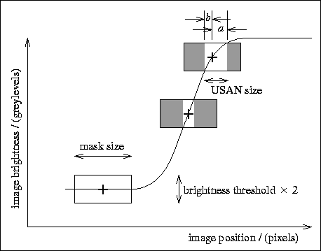
Figure 7: A
monotonically increasing one dimensional input signal and three mask
positions showing USAN size varying with signal gradient. The USAN is
shown as the white portion of the mask. The mask centred on the signal
inflection has the smallest USAN.
If we have general image position x, image function  and
brightness threshold t, then a and b (the ``right'' and ``left''
widths of the USAN -- see Figure 7), for any specific
image position
and
brightness threshold t, then a and b (the ``right'' and ``left''
widths of the USAN -- see Figure 7), for any specific
image position  , are, by definition, given by

and

The SUSAN principle is formulated in the following equation, where
 is the USAN size at
  (the size being a length in
this one dimensional case);
(the size being a length in
this one dimensional case);

assuming that a check is made for n being a minimum and not a maximum. This gives

giving

that is,

unless the image function is constant, an uninteresting case. This is equivalent, in the continuous limit (that is, as t tends to zero), to

and we have equivalence between the two definitions of exact edge position.
This mathematical equivalence in no way means that the SUSAN edge finding method is performing the same function as a derivative based edge detector. No derivatives are taken; indeed, no direction of maximum gradient is identified (in order for differentiation to be performed) in the first place. However, the preceding argument shows why the SUSAN edge detector gives edges to good sub-pixel accuracy even with edges that are not perfect step edges.
It can be seen from the preceding discussion that the initial response of the SUSAN edge detector to a step edge will be increased as the edge is smoothed. The response is also broadened.
As mentioned earlier, the form of the brightness comparison function, the heart of USAN determination (Equation 4), can be shown to achieve the optimal balance between stability and enhancement. This is equivalent to satisfying the criterion that there should be a minimum number of false negatives and false positives. This criterion is formulated in the following expression:

where F is proportional to the number of false positives and false
negatives that will be reported, s is image noise standard
deviation,  is the SUSAN response strength with no edge present
and
is the SUSAN response strength with no edge present
and  is the SUSAN response strength when the mask is centred on
an edge of strength d. Thus this expression simply divides the
expected total ``noise'' by the expected ``signal'' in the most
logical way.
is the SUSAN response strength when the mask is centred on
an edge of strength d. Thus this expression simply divides the
expected total ``noise'' by the expected ``signal'' in the most
logical way.
The value of F will depend on the relative values of d, t and
s. Thus fixing t at 1 and varying the other two variables will
cater for all eventualities. If this expression is averaged over all
likely values of d and s, the overall quality can be evaluated.
The (wide) ranges of d and s chosen were  and
and  respectively; the
reason for choosing the the upper limit on s will shortly
become apparent.
respectively; the
reason for choosing the the upper limit on s will shortly
become apparent.
All of the calculations within the SUSAN feature detectors are based around the use of the equation

where I is defined as before. If the image noise is Gaussian with
standard deviation s then the noise on  will also be
Gaussian with standard deviation
will also be
Gaussian with standard deviation  . Thus F is evaluated over the interval
 .
.
To evaluate F given d, t and s, it is necessary to find the
expectation values and variances of  and
and  , using


and

where

and

with J being the even number determining the shape of the brightness
comparison function; it is 2 for a Gaussian and infinity for a square
function. (N and S are responses due to individual pixels with no
edge present and across an edge respectively, using the brightness
comparison function. The form of  arises from the fact that in
the presence of an edge, half of the response will be due to noise
only, and half of the response will be due to the edge as well as
noise.) The expectation values and variances are computed using the
integrals:
arises from the fact that in
the presence of an edge, half of the response will be due to noise
only, and half of the response will be due to the edge as well as
noise.) The expectation values and variances are computed using the
integrals:
and

where the integral includes the Gaussian model of noise. The integrals
are calculated over the intervals of d and  specified and the mean result for F is thus found. The
resulting plot of F against J is shown in
Figure 8.
specified and the mean result for F is thus found. The
resulting plot of F against J is shown in
Figure 8.
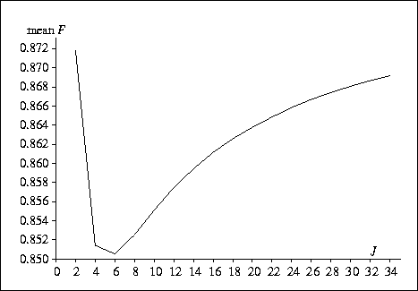
Figure 8: A plot of an objective formulation of expected false
negatives and positives against the J factor in the brightness
comparison function.
It is clear that the optimal value for J is 6. This gives the form of the function used in the SUSAN filters.
The optimal value for g, the geometric threshold, is found by
calculating the mean expectation value for N over the same realistic
range of image noise as before. With no noise present,  is 1;
its mean value in the presence of noise is calculated (using the
integral shown in Equation 24) to be close to
0.75. Therefore the value of g which is likely to provide the
correct amount of noise rejection is
is 1;
its mean value in the presence of noise is calculated (using the
integral shown in Equation 24) to be close to
0.75. Therefore the value of g which is likely to provide the
correct amount of noise rejection is  of the maximum possible
USAN size.
of the maximum possible
USAN size.
Finally, the spatial part of the filter is of interest. In [9] the ``difference of boxes'' edge detector is compared unfavourably with a ``derivative of Gaussian'' edge detector, due to the sharp cutoff in the spatial profile of the ``box'' filter. Because the Gaussian based filter has smooth edges, image noise is suppressed more effectively than using a box (or square) shaped filter. Therefore it may seem that a similar approach to the design of the mask used in SUSAN feature detection would be preferable. Indeed, in the brightness domain, it was found worthwhile to use a smooth brightness comparison function (as shown in Equation 4), rather than having thresholding done with a sharp cutoff. In the case of the spatial extent of the mask, the equivalent process would be achieved by using
in place of Equation 2, where  is a suitable
scaling factor. This would give a circular mask with pixels
contributing less to the calculations as their distance from the
nucleus increased -- a Gaussian profile. An edge detector based on
this kind of mask has been fully implemented and tested.
is a suitable
scaling factor. This would give a circular mask with pixels
contributing less to the calculations as their distance from the
nucleus increased -- a Gaussian profile. An edge detector based on
this kind of mask has been fully implemented and tested.
The difference in practice between the Gaussian spatial SUSAN detector and a sharp cutoff SUSAN detector turns out to be minimal; there is very little difference in the final reliability or localization of reported edges. The explanation for this possibly surprising result is that, unlike the differential edge detector, no image derivatives are used, so that the problem of noise is vastly reduced in the first place. Also, a linear filter is performing a different task to the initial SUSAN response. In the former, a filter has a Gaussian profile in a ``brightness versus distance'' plot. However, the latter uses either a sharp circular mask or a Gaussian profile in the spatial domain and smoothed thresholding in the brightness domain. Thus ``half'' of the algorithm already has a smooth cutoff action. From the results, it seems that it is this part (the brightness domain) which is more important. Thus it does not appear necessary to use a Gaussian spatial mask, although it is easy to do so if desired.

