In edge detection the exact position of an edge is fairly well defined. However, as explained earlier, the exact position of a two dimensional feature is more subjective. Thus there is no strong reason why mathematical understanding of how the SUSAN ``corner'' detector works should give any more validity to the algorithm than the ``intuitively picturesque'' descriptions already given, or an analysis of results. However, a brief mathematical analysis of the algorithm is now given.
For a corner to be detected, a local minimum in n must be found;

that is, differentiating with respect to both components of
 must give zero. (n must also be below the geometric
threshold. This is accounted for later.) Thus, using
Equations 4 and 2 we have
must give zero. (n must also be below the geometric
threshold. This is accounted for later.) Thus, using
Equations 4 and 2 we have

where  is the elemental area within the mask. (The summation
has been replaced by a double integral to clarify the analytical
approach later.) This gives on differentiation
is the elemental area within the mask. (The summation
has been replaced by a double integral to clarify the analytical
approach later.) This gives on differentiation

with B given by

This function B has the property of picking out the narrow bands
that lie on the boundaries between the univalue regions; it is zero
everywhere apart from fairly sharp peaks centred at I( . See Figure 5(c). In other words, in
the context of this algorithm, it is acting as a region boundary
detector. Figure 19 shows a simplified example of the area
picked out by B.
. See Figure 5(c). In other words, in
the context of this algorithm, it is acting as a region boundary
detector. Figure 19 shows a simplified example of the area
picked out by B.
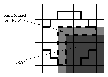
Figure 19: Part of a typical real scene, including a  corner,
with edges slightly blurred. The area picked out by function B is
surrounded by the thick dotted line.
corner,
with edges slightly blurred. The area picked out by function B is
surrounded by the thick dotted line.
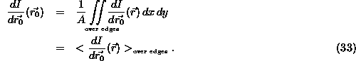
Thus the integral is effectively

giving, on integration,

where A is the effective total area of the narrow bands that make up the edges between the univalue regions (the bands picked out by B). Dividing by A, we have
This equation expresses the fact that the intensity differential at the nucleus must be the same as the intensity differential averaged over all of the boundaries. This must be the case for both the x and y differentials. For this to hold, the nucleus must be placed on a line of reflective symmetry of the boundary pattern within the mask area. This is so that the contributions to the average differential on either side of the nucleus may balance out. This is equivalent to saying that the nucleus must lie on a local maximum in the edge curvature; consider a Taylor's expansion of the edge curvature. At the smallest local level, the nucleus will only lie on a centre of symmetry of the curvature if it lies at a maximum (or minimum) of curvature.
The conditions derived ensure that the nucleus lies not only on an edge, but also that it is placed on a sharp point on the edge. It will as it stands give a false positive result on a straight edge; this is countered by not just finding local minima in n, but by forcing n to be below the geometric threshold g.
Finally, an explanation is needed of why the SUSAN ``corner'' detector is a successful two dimensional feature detector, and not just a simple corner detector. As will be seen shortly, multi-region junctions are correctly reported by the feature detector with no loss of accuracy. This is expected, as the corner finder will look for the vertex of each region individually; the presence of more than two regions near the nucleus will not cause any confusion. (This is a strong advantage over derivative based detectors, where the two dimensional derivative model does not hold at multi-region junctions.) The local non-maximum suppression will simply choose the pixel at the vertex of the region having the sharpest corner for the exact location of the final marker. Thus the different types of two dimensional junction are not in fact seen as special cases at all, and are all treated correctly.