``Noise'' can be introduced into a digitized image in many ways,
starting with the lens of the imaging hardware![]() and ending at the digitization of the captured image.
and ending at the digitization of the captured image.![]() The reduction of noise
without degradation of the underlying image has attracted much
attention in the past. However, whilst many ``structure preserving''
filters have achieved some degree of success at preserving one
dimensional image structure, very few have successfully preserved two
dimensional image brightness structure, such as corners and junctions.
The reduction of noise
without degradation of the underlying image has attracted much
attention in the past. However, whilst many ``structure preserving''
filters have achieved some degree of success at preserving one
dimensional image structure, very few have successfully preserved two
dimensional image brightness structure, such as corners and junctions.
This section describes the SUSAN noise filtering
algorithm.![]() This uses local measurements to obtain noise reduction
whilst preserving both one and two dimensional image structure. The
method is based on image region determination using a non-rigid (in
fact, spatially undetermined) region model.
This uses local measurements to obtain noise reduction
whilst preserving both one and two dimensional image structure. The
method is based on image region determination using a non-rigid (in
fact, spatially undetermined) region model.
The simplest noise reduction method is the sliding mean or box filter (see [35]). Each pixel value is replaced by the mean of its local neighbours. The Gaussian filter is similar to the box filter, except that the values of the neighbouring pixels are given different weighting, that being defined by a spatial Gaussian distribution. The Gaussian filter is probably the most widely used noise reducing filter. It has been incorporated into the design of many algorithms such as the Canny edge detector (see [9]). The Gaussian filter is pleasing because Fourier analysis shows that the Gaussian spatial distribution gives a Gaussian frequency distribution, leading to a good (often described as ``optimal'') tradeoff between localization in the spatial and in the frequency domains. The sharp cutoff of the box filter causes it to give a noisier output than the Gaussian (see the discussion in [9]) corresponding to a less well localized frequency response.
More complicated ``optimal'' statistical estimators have been derived which use local means and autocorrelation functions to calculate the underlying signal (for example Wiener filtering -- see [49]). However, these methods are usually very slow.
Linear filters such as the box and the Gaussian filters tend to create more blurring of image details than do most non-linear filters. An increase in their ability to smooth noise corresponds to an increase in the blurring effect.
Many non-linear filters fall into the category of order statistic neighbour operators. This means that the local neighbours are sorted into ascending order (according to their value) and this list is processed to give an estimate of the underlying image brightness. The simplest order statistic operator is the median (see [69]), where the central value in the ordered list is used for the new value of the brightness. The median filter is much better at preserving straight edge structure than Gaussian smoothing, but if the edge is curved then image degradation occurs. At corners, other two dimensional features and thin lines the median does not perform well with regard to structure preservation. The median is good at reducing impulse noise (for example ``salt and pepper'' noise) where the noisy pixels contain no information about their original values.
There have been several variations on the median filter, for example the weighted median filter (see [7]) selectively gives the neighbouring pixels multiple entries to the ordered list, usually with the centre pixels of the neighbourhood contributing more entries. The higher the weighting given to the central pixel, the better the filter is at preserving corners, but the less the smoothing effect is. At corners, other pixels within the convex image region including the centre pixel are not given any higher weighting than those outside, so this is an ineffective way of preserving the corner structure. Other methods include the contrast-dependent thresholded median (see [55]), adaptive decimated median filtering (see [1]) and the midrange estimator (see [2]), which places the brightness estimate halfway between the maximum and minimum local brightness values.
Three similar filters, the first two of which are typical of more
complicated order statistic operators, are the K-nearest
neighbour operator (see [13]), the  -trimmed
mean (see [5]) and the sigma filter (see
[30]). The K-nearest neighbour operator takes the mean of
the K nearest neighbours from within the ordered list. The value
which K is usually set to (5 or 6 when a 3 by 3 mask is used) means
that corners and thin lines are badly corrupted. The trimmed mean
operator takes the mean of the remaining entries in the ordered list
once the first and last
-trimmed
mean (see [5]) and the sigma filter (see
[30]). The K-nearest neighbour operator takes the mean of
the K nearest neighbours from within the ordered list. The value
which K is usually set to (5 or 6 when a 3 by 3 mask is used) means
that corners and thin lines are badly corrupted. The trimmed mean
operator takes the mean of the remaining entries in the ordered list
once the first and last  entries in the list (originally
containing N entries) have been thrown away. The sigma filter takes
an average of only those neighbouring pixels whose values lie within
entries in the list (originally
containing N entries) have been thrown away. The sigma filter takes
an average of only those neighbouring pixels whose values lie within
 of the central pixel value, where
  is found once for
the whole image. This attempts to average a pixel with only those
neighbours which have values ``close'' to it, compared with the image
noise standard deviation.
is found once for
the whole image. This attempts to average a pixel with only those
neighbours which have values ``close'' to it, compared with the image
noise standard deviation.
The peak noise filter is specifically designed to remove impulse or peak noise. A pixel's value is compared with the local mean. If it is close then the value remains unchanged. If it is very different then the pixel's value is replaced by the local mean. A more advanced version of this takes a weighted mean of the central value and the local mean, the weighting depending on the difference between these two quantities and also on the local brightness variance. This is similar to the contrast-dependent thresholded median filter, and again, is not very good at structure preservation.
In [47] Perona and Malik use local image gradient to control anisotropic diffusion; smoothing is prevented from crossing edges. This is, in a sense, an opposite approach to the K-nearest neighbour, sigma and SUSAN filters, which work out which neighbours to include in smoothing; anisotropic diffusion works out which neighbours to exclude. In [54] Saint-Marc et al. ``refine and generalize'' the approach of Perona and Malik, using many iterations of a 3 by 3 mask which weights a mean of the neighbours' values according to the edge gradient found at each neighbours' position. This method shall be referred to as the SMCM filter. Because pixels both sides of an edge have high gradient associated with them, thin lines and corners are degraded by this process. This problem is also true with Perona and Malik's method. Biased Anisotropic Diffusion (see [44]) uses physical diffusion models to inhibit smoothing across boundaries, according to a cost functional which attempts to minimize a combination of desired components. These individual costs are image smoothness and quality of fit between original and smoothed image. This type of approach is similar to the weak membrane model (see [6]) which fits a membrane to the image surface, allowing it to ``break'' at significant discontinuities, incurring a cost, which is balanced against the ``badness of fit'' cost. This method tends to be very computationally expensive.
Specific surface model fitting techniques have been developed; for example, in [59] a two stage surface fitting method is used. In the first stage a moving least median of squares of errors of a fit to planar facets is used. This is similar to a least mean squares fit to a plane, but uses the median of the errors instead of the mean so that discontinuities are correctly fitted. However, corners are rounded, as with the standard median smoothing; this is expected, and can be clearly seen in the results presented. The second stage fits a weighted bicubic spline to the output of the first stage. As with this approach in general, the success is limited by the model used; image structure not conforming to the model will not be well preserved.
Morphological noise suppression, using mathematical morphology, is related to order statistic neighbour operators. In [43] this type of operator is discussed and compared with other filters. Noble reports that morphological filters perform worse than the moving average and median filters for Gaussian type noise and slightly better than these for ``salt and pepper'' noise.
The hysteresis smoothing approach (see [17]) follows positive and negative gradients in the image, only allowing changes in the gradient when the change is significant, i.e., the new gradient continues further on in the image. The results of using this approach, tested in [24], were not very encouraging, showing a decrease in the signal to noise ratio with each of four different types of noise.
The selected-neighbourhood averaging (e.g., see [40]) method chooses a local neighbourhood to smooth over based on a variety of criteria. Each pixel can be part of several different ``windows''; the one chosen to smooth over is the most homogeneous window which contains the pixel in question as part of its homogeneity. Various window shapes have been tried. These methods are limited to succeeding only on those parts of the image which obey the model used. Sharp corners, for example, will not be correctly dealt with by a square window. A variation on these algorithms is the use of a thin window which is perpendicular to the direction of maximum gradient. Clearly the structure preserving success of this is limited to relatively straight edges.
The symmetric nearest neighbours (see [27]) approach takes each symmetric pair of neighbouring pixels and uses the closer value to the centre pixel from each pair to form a mean output value. Again this is not well suited to preserving corners.
In [31] three methods of noise reduction using different local image measurements to avoid destroying image structure are presented, all based on the assumption that image regions bounded by edges have constant value. In the first method, image edges are found, and for each image position the local edge structure is matched to a list of binary templates which attempt to cover all possible straight edge configurations. Each template has a corresponding weight matrix which determines which elements of the local neighbourhood should be used for smoothing. The system attempts to cope with junctions by taking a convex combination of the different matrix outputs, each weighted according to the quality of the match between the actual local edge configuration and the template. This process is applied iteratively. Although edge structures are well preserved, corners are rounded and ramps are flattened. In the second method the local image gradient is calculated in several different directions, and the results of this are combined to give a smoothing matrix which attempts to smooth only over the bounded constant image region which includes the central pixel. Again, this is applied iteratively. The second method suffers from the same problems as the first method. The third method uses probabilistic relaxation where each pixel has a probability distribution amongst the entire set of possible values, thus vastly increasing the data set. The initial distribution is assumed to be Gaussian. Relaxation is then used to allow the pixels' distributions to interact to find a stable best estimate of the underlying signal. The results given suggest that this method does not in general work as well as the first two.
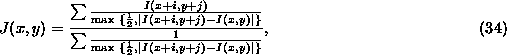
The gradient inverse weighted operator (see [73]) forms a weighted mean of the local pixels, with the weights depending on the difference between the central pixel's value and the value of the local pixels;
where  is the original image,
  is the smoothed image,
and the summation is taken over a 3 by 3 square neighbourhood. The
filter is applied iteratively, typically five times. No preset
threshold is needed. This method reduces Gaussian noise well whilst
preserving image structure. Impulse noise would be much better dealt
with if the central pixel were excluded from the two sums in
Equation 34, for obvious reasons, but this was not included
in the method.
is the smoothed image,
and the summation is taken over a 3 by 3 square neighbourhood. The
filter is applied iteratively, typically five times. No preset
threshold is needed. This method reduces Gaussian noise well whilst
preserving image structure. Impulse noise would be much better dealt
with if the central pixel were excluded from the two sums in
Equation 34, for obvious reasons, but this was not included
in the method.
Finally, image averaging using many images of the same scene (taken quickly one after another) has been used to reduce image noise. For example, see [57]. However, for many image processing applications this approach is impractical; the camera may be moving, the scene may be changing, and it may be necessary to use every image in its own right.