Example 3: Perfusion Analysis using multi-PLD pcASL (GUI)
Introduction
The purpose of this example is to analyse data that has been acquired with multiple post-labeling delays. The analysis is on data from the same subject (and the same session) as used in Example 1 and Example 2. This example uses the data first met in Chapter 4 of the primer.
NOTE that we reccomend you use FSL v6.0.1 (or higher) for these exercises.
For this example you should use the Multi-PLD pcASL data, you will also need images from the Single-PLD pcASL data. The multi-PLD pcASL data was acquired using a label duration of 1.4 seconds and PLDs of 0.25, 0.5, 0.75, 1.0, 1.25 and 1.5 seconds.
Get the data
Perfusion Quantification
(Primer Example Box 4.1)
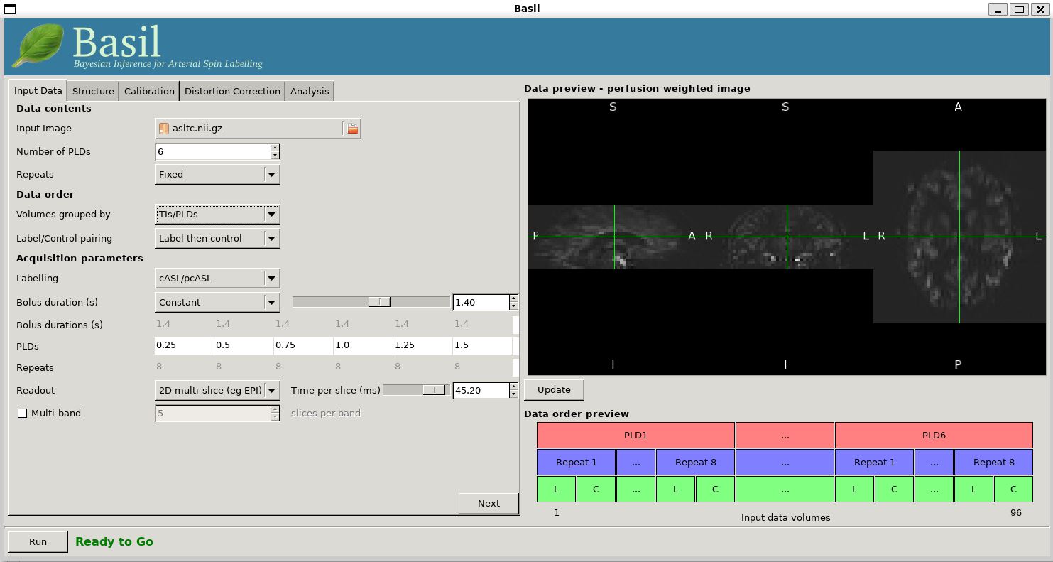
Load the GUI (Asl or Asl_gui). On the
'Input Data' tab, for the 'Input Image' load
asltc.nii.gz. Unlike the single-PLD data in Example 1 we need to specify the correct number
of PLD, which is 6. At this point the 'Number of repeats' should
correctly read 8. Click 'Update' below the 'Data preview pane'. A
perfusion-weighted image should appear - this is an average over all
the PLDs (and will thus look different to Example 1).
Note the 'Data order preview'. For mutli-PLD ASL it is important to get the data order specification right. In this case the default options in the GUI are not correct. The PLDs do come as label-control pairs, i.e. alternating label then control images. But, the default assumption in the GUI is that a full set of the 6 PLDs has been acquired first, then this has been repeated 8 subseqeunt times. (This is quite commonly how multi-PLD ASL data is acquired, but that might not always be how the data is ordered in the final image file) .
As we noted earlier, in this data all of the measurements at the same PLD are grouped together. You need to change the 'Volumes Grouped By' option to 'TIs/PLDs' on the 'Input Data' tab. Note that the data order preview changes to reflect the different ordering. This is now correct: we have 8 repeats of the first PLD followed by 8 repeats of the second, and so on.
Note that if you were to click 'Update' on the 'Data preview' nothing
changes, the ordering doesn't affect the (simple) way in which we
have calucated the PWI. Getting a plausible looking PWI is a good sign that the data
order is correct, but it is not a guarantee that the PLD ordering is
correct, so always check carefully. One way to do this, in this
case, would be to open the data in fsleyes and look at
the timeseries: the raw intensity of both label and control images
for one PLD are different to those from another PLD (due to the
background suprresion). The timeseries for the raw data looks like a
series of steps, indicating the repeated measurements from each PLD
are grouped together (groubed by 'repeats').
- Once we are happy with the PWI and data order, we can set the
'Acquisition parameters':
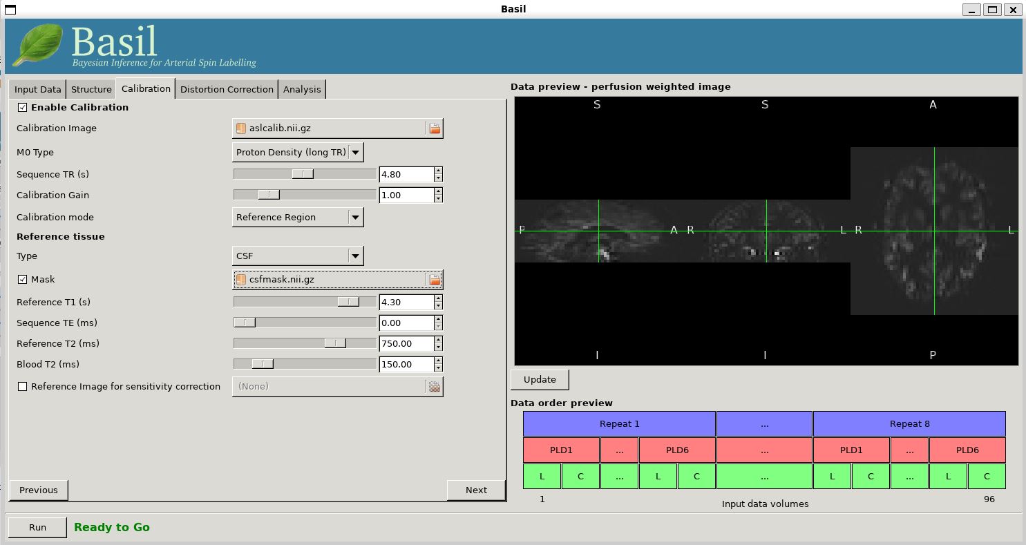
Move to the 'Calibration' tab, select 'Enable Calibration' and as
the 'Calibration Image' load the aslcalib.nii.gz image
from the Single-PLD data (it is from the same subject in the same
session so we can use it here too). We have skipped the 'Structure'
tab (to make the analysis quicker), this means if we want 'Calibration
mode' to be 'Reference Region' we need to supply a 'Mask' of the
region of tissue to use. This has been supplied with this data (in fact
it is simply the result of running the analysis from Example 2). You should select 'Mask' and load
csfmask.nii.gz. Set the 'Sequence TR' to be 4.8, but
leave all of the other options alone.
Move to the 'Distortion Correction' tab. Select 'Apply disotrion
correction'. Load the 'Phase-encode-reveresed calibration image'
aslcalib_PA.nii.gz from the Single-PLD pcASL data. Set the 'Effective EPI echo
spacing' to 0.00095 and the 'Phase encoding direction' to 'y'.
Finally, move to the 'Analysis' tab. Choose an output directory, leave all of the other options alone. Click 'Run'.
The results directory from this analysis should look similar to
that obtained in Example 2. The main difference is that the
arrival.nii.gz image is now a genuine estimate of
ATT; if you examine this image you should find a pattern of values
consistent with the time it takes for blood to transit between the
labeling to imaging regions. You might notice that the
arrival.nii.gz image was present even in the single-PLD
results, but if you looked at it contained a single value - the one
set in the Analysis tab - which meant that it
appeared blank in that case.
Arterial/Macrovascular Signal Correction
(Primer Example Box 4.2)
In the analysis above we didn't attempt to model the presence of arterial (macrovascular) signal. This is fairly reasonable for pcASL in general, since we can only start sampling some time after the first arrival of labeled blood-water in the imaging region. However, given we are using shorter PLD in our multi-PLD sampling to improve the SNR there is a much greater likelihood of arterial signal being present. Thus, we might like to repeat the analysis with this component included
Return to your analysis from before. On the 'Analysis' tab select 'Include macro vascular component'. Click 'Run'.
The results directory should be almost identical to the previous run, but now we also gain some new results:aCBV.nii.gz and
aCBV_calib.nii.gz; following the convention for the
perfusion images, these are the relative and absolute arterial
(cerebral) blood volumes respectively. If you examine one of these
and focus on the more inferior slices you should see a pattern of
higher values that map out the structure of the major arterial
vasculature, including the Circle of Willis. This finding of an
arterial contribution in some voxels results in a correction to the
perfusion image - you may now be able to spot that in the same
slices where there was some evidence for arterial contamination of
the perfusion image before that has now been removed.
Partial Volume Correction
(Primer Example Box 6.4)
In the same way that we could do partial volume correction in Example 2 for single PLD pcASL, we can do this for multi-PLD.
Return to your analysis setup. We will require structural
information, so go to the 'Structure' tab. We will use the structural
image from the Single-PLD pcASL data (same subject). Either choose
'Structural data from' 'Run FSL_ANAT on structural image' and load the
'Structural Image' from the Single-PLD pcASL data directory, or use
the output of fsl_anat from a previous run with the
'Structural data from' 'Existing FSL_ANAT output', loading the
T1.anat accordingly. On the 'Analysis' tab, select
'Partial Volume Correction'. Click 'Run'.
The results directory now contains, as a further subdirectory, pvcorr,
within the native_space subdirectory, the partial volume
corrected results: gray matter (perfusion_calib.nii.gz
etc) and white matter perfusion
(perfusion_wm_calib.nii.gz etc)
maps. Alongside these there are also gray and white matter ATT maps
(arrival and arrival_wm respectively). The
estimated maps for the arterial component
(aCBV_calib.nii.gz etc) are still present in the
pvcorr directory. Since this is not tissue specific there
are not separate gray and white matter versions of this parameter.