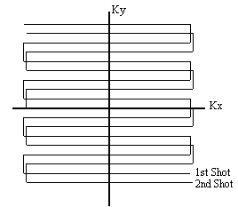
Interleaved EPI acquires all the data points required to make up the image in several FIDs. The easiest way to picture how this is done is to look at the k-space coverage diagram (Figure 5.1) for a two shot interleaved EPI sequence. The first interleave covers the whole of k-space in alternate lines, and then the second pass fills in the lines between. The same principle holds for any number of interleaves, up until the technique essentially becomes a 2DFT experiment.
The technique is sometimes referred to as segmented EPI, since k-space is covered in two or more segments. There are other ways that k-space can be segmented, for example, acquiring the positive ky values in the first shot, and negative values in the second. It seems appropriate to refer to the kind of technique shown in Figure 5.1 as interleaved EPI, since the two shots are indeed interleaved on reconstruction, and to refer to other multi-shot techniques as segmented EPI.
The pulse sequence diagram required for two shot interleaved EPI is shown in Figure 5.2. Both shots are essentially MBEST modules, but with three differences between the first and second shot. Firstly there is a difference in the length of the pre excursion of the blipped gradient. This ensures that the phase encoding is slightly different for each shot, so that every line of k-space is acquired. Assuming that the magnitude of the blipped pre-excursion gradient is the same as the blipped gradient itself, then the excursion must increase in length by half of the duration of one blip, for each interleave. Since increasing the length of the pre-excursion delays, albeit slightly, the time of the echo, an appropriate delay must be added in the earlier interleave to compensate.
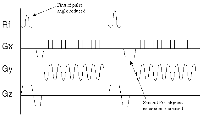
The other two differences relate to discontinuities in the phase and magnitude of the signal along the ky direction in the final image.
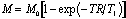
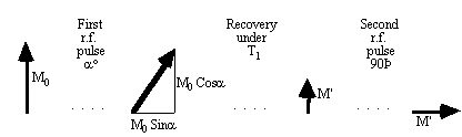
The second difference between shots in the pulse sequence diagram relates to the magnitude of the transverse magnetisation vector after the r.f. pulse. If the magnitude of the longitudinal magnetisation prior to the experiment is M0, then following a 90 degree pulse the transverse magnetisation will be M0, and the longitudinal magnetisation will be zero. In the duration, TR, between the first and second r.f. pulses the longitudinal magnetisation will recover through T1 relaxation, and following a second 90 degree pulse the transverse magnetisation will be
 .
.
(5.1)
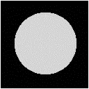
Unless TR >> T1, the signal intensity of the two interleaves will therefore be significantly different. This leads to discontinuities in k-space and causes ghosting artefact, as demonstrated in Figure 5.3. The effect can be compensated for by reducing the flip angle of the first pulse.
 (b)
(b) 
The z-magnetisation prior to the nth interleave is given by

(5.2)
and for constant signal following each excitation
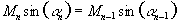 .
.
(5.3)
These equations can be solved iteratively, with the last flip angle being 90 degree, to find the flip angles for each of the interleaves. These equations only hold for one value of T1, and so discontinuities between interleaves in the signal from tissue with a different value of T1 will still occur. To reduce this problem McKinnon suggests calculating a slightly longer series than necessary, and only using the first part of the series [4].
In using interleaved EPI for fMRI, many images are obtained with a constant repetition rate. This means that a constant flip angle can be used, and after the first few images have been acquired the magnitude of the longitudinal magnetisation reaches a steady state.
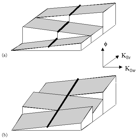
The third difference in the pulse sequences between interleaves, acts to reduce phase discontinuities in the time data. Off-resonance phase errors, due to field inhomogeneity, susceptibility and chemical shift, evolve constantly with time. Since in each interleave alternate lines are acquired under opposite read gradients, these lines must be reversed in the time data matrix prior to Fourier transformation. This leads to steps in the phase, which may cause ghosting artefact. This can be a problem in conventional EPI, but the problem is compounded in N shot interleaved EPI, since the first N lines are all acquired at the same time in the echo train, and thus the steps are N times longer (see Figure 5.4a).
To compensate for this, at least along the central line of k-space, a slight time delay of magnitude

(5.4)
is added to the nth interleave (Tx is the time needed to acquire one line in k-space). This has the effect of smoothing out the discontinuities (see Figure 5.4b) [5,6].
Since it is commonly required to image several slices when carrying out an fMRI experiment, the signal to noise ratio can be improved by employing a multi-slice technique. The k-space diagram for multi-slice interleaved EPI is shown in Figure 5.5.
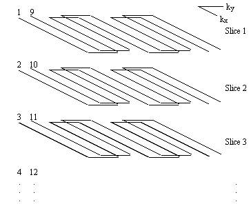
The first shot of every slice is acquired before returning to acquire the second interleave. This increases the steady state transverse magnetisation available after each pulse, and therefore increases the signal to noise ratio.
The benefits are slightly offset by the risk of subject movement during the acquisition. If the movement occurs between the first and second shot of one slice, that image will show artefact as a result. The chances of this occurring is much greater if there is a long delay between shots, as is the case in the multi-slice experiment.