As was described in Chapter 3, task performance causes a local increase in the value of T2* in the region of the brain that is involved in the task, which can be detected in T2* weighted images. The amount of T2* weighting that is seen in an image depends on the echo time, TE (see section 2.4.2). For a given value of T2*, images obtained with a value of TE equal to T2* will be optimal at detecting any change in T2* (see section 3.3.3). The magnitude of T2* depends on a number of factors that are scanner dependent, such as field strength and quality of shimming, and others that are object dependent, such as the orientation of the boundaries between regions with differing magnetic susceptibility.
Given this, it becomes important to find the value of TE which will give the best detection of even the smallest changes in T2* in the region of brain that is being studied. This has been done previously by carrying out several experiments, each using different echo times [1]. Changes in the value of T2* upon visual activation have also been measured using spectroscopy [2], and multi echo FLASH [3]. More recently, a double echo time approach to T2* mapping has been demonstrated [4]. Here, a technique is presented which obtains a set of low resolution images with six different echo times from a single FID. This enables activation images from each different echo time to be obtained for precisely the same task. By fitting T2* curves to the data, it has also been possible to obtain maps of T2* during activation. This sequence has been used in activation experiments involving visual and auditory stimulation, and motor tasks on five normal volunteers.
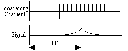
In EPI, a gradient echo is formed in the broadening direction by applying an initial dephasing gradient, and then a series of 'blips' of the opposite polarity which form the echo. The time from the r.f. excitation pulse to the centre of the echo is defined as the echo time in EPI (see Figure 4.1). This is distinct from the repeated set of echoes formed by the switching of the read gradient.
Having formed one gradient echo, it is possible to form other echoes simply by reversing the polarity of the blipped gradient. These echoes all form under the T2* decay envelope, and have different echo times (Figure 4.2). This is distinct from the multiple spin echo experiment described in section 2.4.3, in which the echoes form under the T2 decay envelope.

The signal can continually be recalled in this way, provided that T2* has not already reduced the signal to zero.
The above sequence was implemented on a dedicated EPI 3.0 Tesla scanner, with purpose built head gradient coils, birdcage r.f. coil, and control. In order to sample at 6 echo times between 10 and 55 ms, a matrix size of 32 x 32 and a switching rate of 1.9 kHz was chosen. This gave echo times of approximately 12, 20, 28, 36, 44 and 52 ms, and a voxel resolution of 5 x 5 x 10 mm3. The ordering of the rows in the 2nd, 4th and 6th echo time image was reversed prior to Fourier transformation to maintain the equivalent orientation of the images.
A T2* map was calculated for every FID by fitting the data from each echo time, on a pixel by pixel basis, to an exponential decay curve of the form
![]() .
.
(4.1)
This was done by taking the logarithm of the pixel intensity and calculating the linear regression, intercept and correlation coefficients between these and the echo time. These values were used to form images of T2*, S0 and correlation.
The activation experiments were designed to produce a response in the visual, motor and auditory cortices. For the visual and motor experiment, the subject observed an LED display. During the task condition, an outer ring of LED's lit, and a central bar flashed at a rate of 2 Hz. The subject was required to respond to the stimulus by pressing a hand held button at the same rate as the flashing LED. The whole brain was imaged, in 16 slices, every 4 seconds. The experiment consisted of 16 seconds of rest followed by 16 seconds of activity, repeated 32 times, and was carried out on 5 normal volunteers.
The auditory experiment consisted of imaging 6 slices through the temporal lobes in 600 ms, each set of slices being acquired every 14 seconds. In alternate gaps, a 14 second recording of speech was played to the subject. Thus for each cycle one volume set of images was obtained directly after a 14 second period of auditory stimulation, and one set was acquired after a 14 second period of silence. The advantage of carrying out the experiment in this way is that the auditory stimulation from the scanner does not interfere with the auditory stimulation of the speech. Each experiment consisted of 20 cycles of speech and silence, and was carried out on 5 normal volunteers.
The analysis of the data was carried out using the techniques and software described in Chapter 6. Following image formation, the echo time data was normalised, spatially filtered with a 3D Gaussian kernel with FWHM of 6 mm, and temporally filtered with a Gaussian kernel of FWHM 3 s. For the visual and motor experiment the time course was correlated to a delayed and smoothed reference waveform (square wave convolved with a Poisson function with l = 6 s), on a pixel by pixel basis to produce one statistical parametric map (SPM) for each echo time.
The auditory activation data was analysed using a t-test comparison between the mean of the speech and silence images, again forming one SPM for each echo time. The correlation coefficients and t-scores were transformed to z-scores and thresholded to the same p-value using both peak height and spatial extent of the SPM.
For each echo time, the mean percentage change between activation and rest was calculated, for all the pixels in the active regions. In order to ascertain which echo time yields the optimum results, the product of the mean percentage change and the number of pixels in the activated region was calculated.
Similar statistical analysis was performed on the T2* maps.
Examples of the activation images produced, for each echo time and for the T2* maps, are shown in Figure 4.3. The colours in the active regions refer to the level of percentage change in each region, and these are overlaid on the mean of the images acquired at that echo time. The levels of significance of the activation (p value) were less for the T2* maps than for the T2* weighted images, however discrete regions of activation in the same regions can be seen. The general trend is for the percentage change to increase with echo time, however the extent of the activation detected reduces with the longer echo times. This is illustrated in the graphs of the product of percentage change and number of active pixels, shown in Figure 4.4 for each of the subjects. The dotted line on these plots represents the activation from the T2* maps. The level of percentage change observed in the T2* maps upon activation was usually greater than that observed in the T2* weighted images, but the regions were generally smaller. No significant change was detected in the maps of S0 during the tasks.
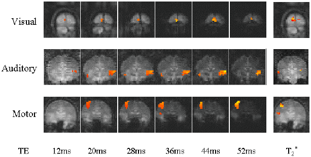
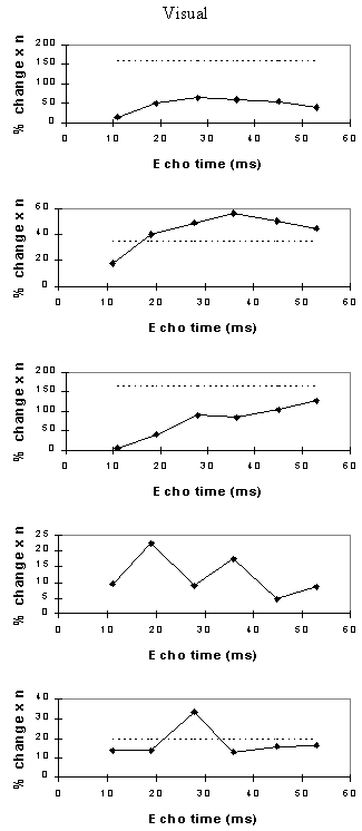
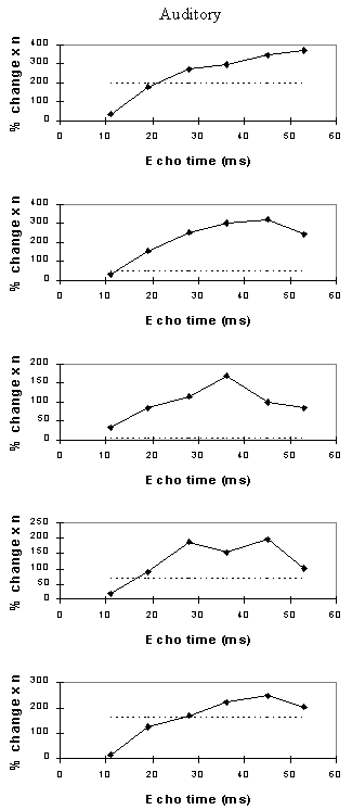
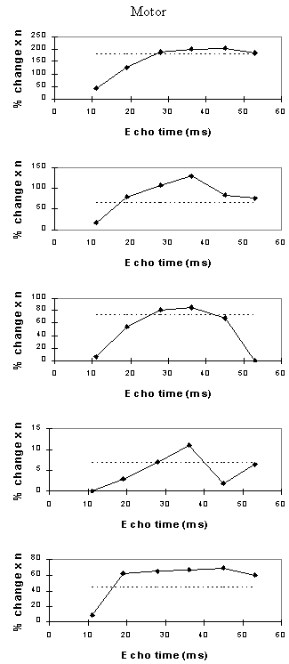
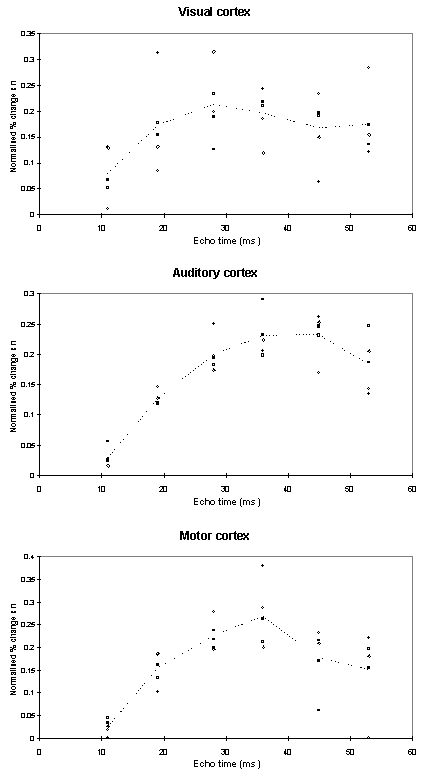
An appropriate choice of echo time for the motor and auditory cortices, would appear to be between 30 and 40 ms, and between 25 and 35 for the visual cortex. If the echo time is too short, the percentage change is so small that the activation response is lost in the contrast to noise of the time series. However if the echo time is too long, the signal from the cortex has fallen to zero due to T2* decay and no change is seen on activation.
The multiple gradient echo technique produces, from a single FID, a set of images with different values of echo time. Measuring several echo times in one experiment has the advantage of reducing the total experimental duration, and eliminating the effects that habituation, subject restlessness, or repositioning could have on the results if separate experiments were carried out at each echo time. The results suggest that an echo time of between 25 and 40 ms would be optimum for experiments in the visual, motor and auditory cortices at 3 T. More results would be required in order to be confident of using a similar echo time for studies in other regions of the brain, but this technique offers a quick and simple way to carry out such an experiment.
The relatively thick slices used, will mean that through slice dephasing will reduce the values of T2*. The slice thickness of 10 mm used in this experiment is comparable to that used in many whole brain studies, however the choice of optimum echo time may be different for the thinner slices used in some experiments.
The use of T2* maps, instead of T2* weighted images for fMRI has the additional benefit that the results will not be so affected by in-flow effects, or through slice movement artefact. If higher resolution images were required, the number of echo times recorded could be reduced, so that the number of lines in the image could be increased. For example four 64 x 64 images could be acquired with echo times of 16, 32, 48 and 64 ms, and T2* curves fitted to this data, allowing an in plane resolution of up to 3 mm.