The next step after flow estimation is to segment the flow list into
clusters which represent different objects in the
world.![]() The flow within
each cluster is fit to a linear space dependent (i.e., affine) model,
giving a total of six parameters for each cluster, using a
least-squares fit.
The flow within
each cluster is fit to a linear space dependent (i.e., affine) model,
giving a total of six parameters for each cluster, using a
least-squares fit.
The vector values used for the segmentation process may either be the current velocity estimate for each feature, or the feature's displacement over the past N frames, where N is constant, and typically set to 10. The former, more traditional, approach gives results which are more recently accurate, i.e., more ``up-to-date'', whilst the latter is more robust, and usually gives greater discrimination between objects with only slightly differing motion. It is the latter which is usually used within ASSET-2 to create the motion vector field.
The list of flow vectors is processed to find separate clusters using
simple segmentation similar to the concept of the minimum spanning
tree [13]. Each new candidate vector is compared with the
value expected by the running flow model. When a new cluster is
started, the initial flow model is that of constant flow, i.e., two
parameters; this is replaced with the affine model once enough vectors
have been included into the cluster. The distance function used for
comparing a candidate flow vector  with the vector
 estimated by the current model at the candidate flow
vector's position allows small vectors to be matched to each other
without bias by including a noise term into the fractional vector
error;

where  is of the order of the error estimate of the flow
vector. The ``distance'' thus calculated between a new flow vector and
 must be less than a threshold
  for the new vector to be included in the current
cluster. The clustering process terminates when no more ``linkable''
neighbours can be found for any member of the cluster. A new cluster
is then started. There is no question at this stage of ensuring that
clusters do not overlap; the clusters are found individually, and once
a flow vector has been used it is removed from the list.
Finally, once the list of independent clusters of flow vectors has been found, each cluster has its bounding box, centroid and motion model calculated, and added to the cluster description. (The centroid calculated is the mean position of the flow vectors which make up the cluster. This has more meaning than some ``centre of shape'' centroid, as outlying vectors -- vectors incorrectly joined to the cluster -- will not have so great an effect on the centroid.) This information is then passed on to the part of ASSET-2 which tracks clusters over time.
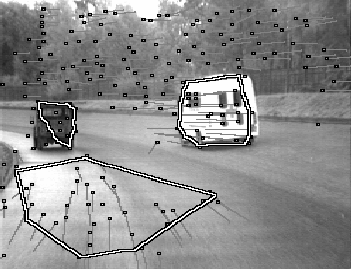
Figure 4 shows a typical set of clusters found by the

Figure 4: An example set of clusters found by the flow segmentation
stage of ASSET-2, superimposed over the flow vectors.
flow segmentation stage of ASSET-2. No cluster has been formed where a flow vector has no neighbours to form one. Note the small errors in the two important clusters, particularly in the Landrover cluster, which should be filtered out over time. The cluster in the foreground will not appear in the filtered cluster list as a ``good'' cluster (see the following section) because it will not be consistent over time. The background cluster is ignored here by the display part of ASSET-2.
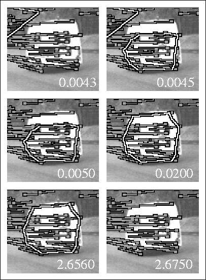
Figure 5 shows the set of clusters found near the ambulance

Figure 5: The clusters found near the ambulance when the segmenting
threshold is varied over a wide range. The value of the threshold is
shown for each case in the bottom right hand corner of the image.
when a variety of values for  is used. It is usually left at 0.15. The results show
in this case that variations in
  of one order of magnitude in either direction are
acceptable, which is an encouraging result for a threshold.