Previous work at DRA Chertsey has used, as input data to calculations of the ``driveable region'' (or ``the road''), local interpolated surface normals, three dimensional height values taken in a fixed global three dimensional co-ordinate frame and positions in the camera's local three dimensional co-ordinate frame. All three of these data types can be computed from the output of DROID. The use of local interpolated surface normals was not very successful due to high noise sensitivity. Because local surface direction depends on the vector differences of three dimensional positions and the other two methods use these positions directly, any noise will naturally become more damaging in the former case. The use of a local three dimensional co-ordinate frame is obviously more robust than a single fixed co-ordinate frame over long image sequences, as there is no susceptibilty to any accumulation of error in the estimated camera position.
The model which is fit to the data must balance the need to accommodate all possible variations within accepted driveable regions with the need to constrain the model to give maximum stability. In other words, the number of degrees of freedom must be not too large and yet not too small. Previous work at DRA Chertsey used a constant height model (one degree of freedom) and a planar fit (three degrees of freedom).
The next more complex isotropic model would naturally be a bi-quadratic fit, with six degrees of freedom. However, transverse curvature and road skew are likely to be very low, and the modelling of these would unnecessarily reduce the ability of the model to distinguish driveable features from non-driveable ones. Hence the model used is a planar-quadratic ``ribbon'', with four degrees of freedom, namely height, two slope angles, and longitudinal curvature (see figure 1 for qualitative indications of these parameters).
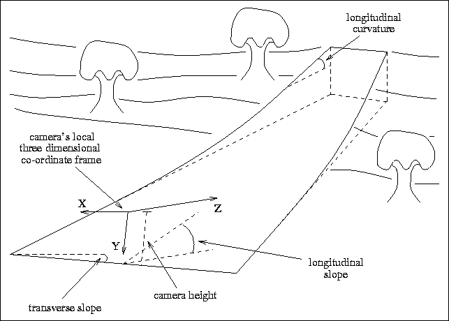
Figure 1: Degrees of
freedom in the planar-quadratic model.
In fact, these four degrees of freedom are slightly constrained; both the curvature and the transverse slope are hard limited to give added stability to the model.
The model is fit to the data using a standard least squares fit, with recursive estimation ignoring outliers. The threshold used for the outlier rejection is set at a constant fraction of the estimated distance between the camera and the road. After computation of the fit in the first frame, the starting position for the fit in subsequent frames is taken as the current estimate of the model parameters. Thus convergence is fast and stable.
Once the best estimates for the four model parameters have been found, they are temporally filtered to improve stability and accuracy, using a simple fixed weight filter (of typical update fraction 0.4). The filtered values are used by the other sections of ALTRUISM, and also, as mentioned above, as the first estimate in the least squares fit for the next frame.
The reason for modelling only the driveable region and not the whole observed scene is that far more constraint can reasonably be put on the expected surface types for the driveable region than for ``off road'' parts of the scene. Also, the non-driveable areas are not of immediate interest to this application, so that as long as the segmentation of driveable and non-driveable points is performed correctly, the non-driveable data can be completely ignored.