This chapter deals with the way in which the raw data from an fMRI experiment is analysed. The aim of such analysis is to determine those regions in the image in which the signal changes upon stimulus presentation. Although it is possible to devise many different techniques for detecting activation, if these techniques are to be used in practice it is necessary to know how much confidence can be placed in the results. That is to say, what is the probability that a purely random response could be falsely labeled as activation. This requires an understanding of the statistics behind the technique used.
Many of the statistically robust techniques used to analyse fMRI data have been developed from PET. These try to model the time course that is expected, and determine how well each pixel's temporal response fits this model. However, since fMRI experiments allow a much greater time resolution than PET, it is possible to carry out experiments which determine the order in which different cognitive events occur. Analysis of the data from such an experiment requires a 'non-directed' technique which makes few assumptions about the timings of the activation responses expected.
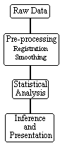
There are three stages to the analysis of the data from any fMRI experiment (Figure 6.1). Firstly there are the pre-processing steps, which can be applied to the data to improve the detection of activation events. These include registering the images, to correct for subject movement during the experiment, and smoothing the data to improve the signal to noise ratio. Next, the statistical analysis, which detects the pixels in the image which show a response to the stimulus, is carried out. Finally the activation images must be displayed, and probability values, which give the statistical confidence that can be placed in the result, quoted.
In order to analyse the data from the experiments explained in Chapter 7, a suite of programs were written, which implement existing and novel analysis techniques for carrying out the steps outlined above. These techniques are described in detail in the following sections.
There are a number of steps that can be carried out prior to the statistical analysis of the data. Each of these steps is independent and offers different benefits. There is an analysis time penalty to be paid for each of the steps, some of which can take times of the order of hours. The theory and implementation of each step is described below, with an integrated package explained in the final section.
The raw time data from the scanner requires Fourier transformation to form the image. The raw data is stored as complex numbers, one for each pixel in the image. Correction for N/2 ghost artefact (see Section 4.3.1) can be carried out at this stage by changing the phase angle between real and imaginary data points of alternate lines. The extent of correction required can be determined by eye, adjusting the phase angle until the N/2 ghost in the first image in the set is minimised. The same correction can then be applied to every image in the fMRI data set. Alternatively one of the methods suggested in Chapter 4 can be utilised. Failure to eliminate any ghost artefact can cause activations from within the head to be aliased in the ghost.
Two dimensional fast Fourier transformation (FFT) is carried out using a standard routine[1], with the images being stored as 4 byte signed integers (shorts). The data is also scaled to utilise the whole range of the short data type (+/- 32767).
Two data reducing steps are performed, which cut down on the number of calculations that need to be carried out. Experimental pre-scans (saturation scans), which ensure that the effects of T1 recovery have reached a steady state, can be removed from the beginning of the data set. Also the matrix size can be reduced so that it covers only the brain.
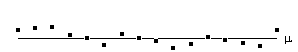
Changes in the global blood flow to the brain (gCBF), as well as instability in the scanner hardware, can cause the mean intensity of the images to vary with time, regardless of functional activity. A plot of the mean intensity of an image of a single slice, acquired every 2 seconds is shown in Figure 6.2.
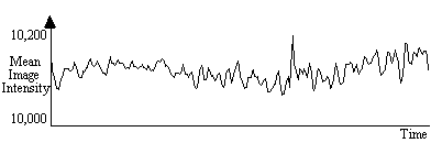
Such fluctuations mean that the response to each stimulus is not identical, and reduces the power of any statistical test performed. In order to remove this effect, each image can be scaled so that it has a mean equal to some pre-determined value, or to the global mean of the whole data set. Since there are fluctuations in the intensity of the artefact caused by external r.f. interference, which are independent of the variation in the true image intensity, it is necessary to exclude these regions from the calculation of the image mean. Regions to exclude are chosen by the user, prior to the normalisation.
Subject head movement, during the experiment is a major source of artefact in fMRI data. Changes in pixel intensity at the edges of the brain, upon even slight movement, can be far greater than the BOLD activation response. It is common therefore in fMRI data analysis to perform some correction which reduces this effect[2].
The approach taken here is to correct only for in-plane translations and rotations of the head within the image. Working on a slice-by-slice basis, the first image is taken to be the reference image, to which all other images of that slice are to be aligned. Two dimensional rotations and translations are applied to the second image, and the sum of the squares of the difference (ssd) between pixels in the first and second image are calculated. Further translations and rotations are applied to the image until the ssd is minimised, using a standard routine. All subsequent images are realigned in the same way.
This technique is quite robust, and does not have difficulty in converging. One obvious extension of this would be to go to a three dimensional technique. This would have the advantage of more fully correcting the head motion, and would also be a faster technique, but introduces the problem of interpolating the data to give isometric voxels. Additional corrections that could be applied include those which remove cardiac and respiratory effects[3], and those which correct for the history of the spins[4].
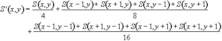
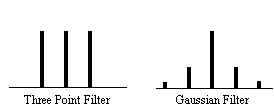
Any reduction in the random noise in the image will improve the ability of a statistical technique to detect true activations[5]. Spatially smoothing each of the images improves the signal-to-noise ratio (SNR), but will reduce the resolution in each image, and so a balance must be found between improving the SNR and maintaining the resolution of the functional image.
The simplest form of smoothing to apply is a 9 point filter, such as the one shown below.

If S(x,y) is the image intensity of a pixel at position (x,y) in the image, then upon applying the above filter this pixel will have value
 (6.1)
(6.1)
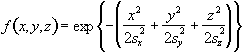
Such a filtering technique is simple and quick, but lacks control of the width of the filter. An alternative is to convolve the image with a three dimensional Gaussian function, of the form
 (6.2)
(6.2)where sx, sy and sz are the standard deviations of the Gaussian in each direction. A good estimate of the extent of such a smoothing is given by the full width at half maximum (FWHM) of the Gaussian kernel. The relationship between standard deviation and FWHM is
FWHM = 2.35s. (6.3)
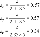
So to smooth an image of resolution 3 x 3 x 5 mm3 with a Gaussian kernel of FWHM 4 mm, the required parameters are
To carry out the filtering, a smoothing matrix is constructed which is the same size as the image. This image matrix is convolved with the smoothing matrix by Fourier transforming both the image and the filter, with a three dimensional FT. Since fast Fourier transformation (FFT) is considerably faster than a discrete Fourier transform, the image and smoothing matrix are zero filled to the nearest 2n points in each direction. The smoothing matrix is scaled so that its maximum point is equal to one, ensuring that the image is not scaled out of the range of the short data type used to store the smoothed image. The two transformed matrices are multiplied together and then inverse Fourier transformed back to give the smoothed image. Such a method of convolution would attempt to smooth the opposite edges of the image with each other, and so zero filling is carried out to the next largest 2n points to prevent this.
There is no straightforward answer to the question of which is the best smoothing width to use in the analysis of the data set. Standard filter theory shows that the best kernel is one which matches the size of the activation region sought. Thus a filter of FWHM of 4 mm would be optimum for regions of this sort of extent, but may reduce the signal from smaller regions (Figure 6.3). A wider filter will reduce the noise to a greater extent, and so a compromise must be reached.
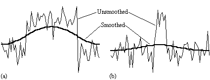
In practice, for most purposes a FWHM of 4 mm is suitable, but larger filters may be useful if the signal to noise ratio is particularly bad, and the activation expected to cover a large area, whilst a narrower filter can be used if the SNR is good enough. An example of the use of three different filters in the analysis of the same data set is shown in Figure 6.4.
(a) (b)
(b) (c)
(c)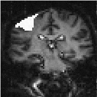
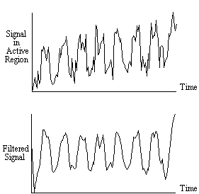
As well as smoothing in the spatial domain, improvements in the signal-to-noise ratio can be made by smoothing in the temporal domain. Since the BOLD contrast effect is moderated by blood flow, the rate at which the signal changes, in a genuinely activated region, is limited. Therefore smoothing each pixel's time series with a filter of similar shape will improve the SNR. From our observations, and figures quoted in the literature[6], a Gaussian of width 2.8 seconds, is a good approximation to the haemodynamic response function, and so this is used to smooth the pixel time courses.
As well as removing the high frequency fluctuations from the time series, it can be beneficial to remove any long term drift that may appear in the data. Such drifts can arise from instability in the scanner hardware, and will reduce the power of the statistical technique in detecting activations.
Both types of temporal filtering are carried out in the Fourier domain. First, an appropriate Gaussian vector, with the same length as the time course, is constructed using the function
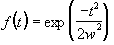 , (6.4)
where w is the width of the Gaussian. This function is Fourier transformed, scaled so that it has a maximum value of one, and the Fourier components from 1 to n-1 are set to zero, where n is the number of cycles in the fMRI experiment. This high-pass filtering will remove low frequency variations in the data, without significantly altering signals correlated to the stimulus. For each pixel in the image, the time course is extracted, Fourier transformed, multiplied by the filter, and inverse Fourier transformed. To use the fast Fourier transform technique it is necessary to have a vector of length 2n. Zero filling can therefore be employed, but it is necessary to subtract the mean from the time course prior to this, to avoid undesirable steps in the data. This mean is added back on to the data after filtering. The effects at the ends of time course must be taken into account, particularly if there is a lot of drift in the data. Figure 6.5 shows an example of a time course taken from a 8 cycle experiment, prior to filtering. Upon filtering, the effects at the edge of the data can be seen. This can reduce the power of the statistical test used, and it might be necessary to exclude the first and last cycles from the statistical analysis.
Experience has shown that care must be taken in using the temporal filtering, particularly in the way that it affects the independence of the data points, a subject covered later in this chapter. However, the improvement in the detection of activation that results, justifies its use.
Each of the above pre-processing steps was coded as a separate 'C' program[7], reading in the data from one file, and outputting it to a new file. Each step takes a reasonable amount of time; a few hours for the registration and tens of minutes for the two filtering steps with data sets of a few thousand images. The programs were therefore joined to form a single pre-processing software suite. The programs were rewritten as functions, with the parameters such as file names and matrix sizes being passed from a main routine. Each step still saves its output in a file, but the software automatically deletes the files once they are no longer required, meaning that less disk space is taken up during the processing. The input parameters for the program are read from an initialisation file. This initialisation file is produced by a separate graphical user interface, allowing the main processing to be run in the background on a UNIX workstation, with no terminal input required once the program is started.
The graphical user interface (GUI) is shown in Figure 6.6. It allows the selection of some or all of the steps to be carried out on the data. Upon completion of each step, the file name is appended with a letter, so that the pre-processing that has been carried out on that file can easily be seen. If all the processing steps are carried out the files will be named
For any image files that are created, a header file compatible with the Analyze display software[8], is also created. Other features of the GUI include the ability to start the processing at a later time specified by the user, and the option to print out the settings used, which can be kept as a record. The GUI was written in 'C', using the xview, library routines. The time taken to pre-process fMRI data is significantly reduced using the new software, largely because all the steps can be set off to run in a few minutes, and allowed to run without the need for user interaction, overnight if necessary.
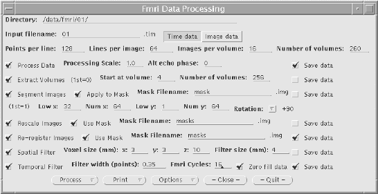
The user instructions for the fMRI pre-processing package is included as Appendix B.
Many techniques have been proposed for statistically analysing fMRI data, and a variety of these are in general use. The aim of such analysis is to produce an image identifying the regions which show significant signal change in response to the task. Each pixel is assigned a value dependent on the likelihood of the null hypothesis, that the observed signal changes can be explained purely by random variation in the data consistent with its variance, being false. Such an image is called a statistical parametric map. The aim of this section is to show how such maps can be produced.
All the methods described below have been used, at one time or another, in the analysis of the data presented in this thesis. The majority have been implemented as 'C' programs, with the notable exception of using the SPM[10] implementation of the general linear model.
Throughout this section, the analysis techniques described are demonstrated on an example data set. The experiment performed was intended to detect activations resulting from a visually cued motor task. The whole brain of the subject was imaged, in 16 coronal slices of resolution 3 x 3 x 10 mm3, every four seconds. As cued by an LED display, they were required to squeeze a ball at the rate of 2 Hz. The experiment involved 16 s of rest, followed by 16 s of task performance, repeated 32 times.
Further detail of the statistics mentioned in this chapter can be found in many statistics text books, for example those by Zar[11], and Miller and Freund[12].
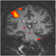
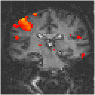
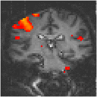
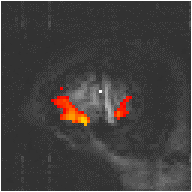
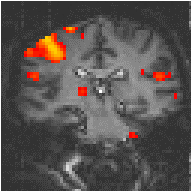
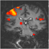
One of the simplest methods for obtaining results from a two state fMRI experiment is to perform a simple subtraction. This is carried out by averaging together all the images acquired during the 'on' phase of the task, and subtracting the average of all the 'off' images. The disadvantage of such a technique is that it is extremely sensitive to head motion, leading to large amounts of artefact in the image. Figure 6.7a shows a single slice through the motor cortex from the example data set, and Figure 6.7b shows the result of subtracting the 'off' images from the 'on' images. Although signal increase can be seen in the primary motor cortex, there is also a large amount of artefact, particularly at the boundaries in the image.
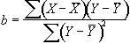
Such a method does not yield a statistic that can be tested against the null hypothesis, so instead of straight subtraction it is more common to use a Student's t-test. This weights the difference in means, by the standard deviation in 'off' or 'on' values, giving high t-scores to large differences with small standard deviations, and low t-scores to small differences with large standard deviations. The t-score is calculated on a pixel by pixel basis, for a time series X, using the formula
 (6.5)
(6.5)
where
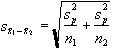 (6.6)
(6.6)
and  is the pooled variance
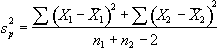 . (6.7)
The suffix '1' refers to the n1 images acquired during the 'on' period of the task, and '2' refers to the n2 images acquired during the rest period. Figure 6.7c shows the statistical parametric map of t-scores for the sample data set. Again motor cortex activation is clearly seen, but the movement artefact is reduced compared to the subtraction technique.
(a)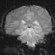 (b)
(b)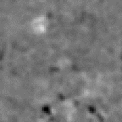 (c)
(c)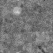
Since we know that the BOLD response is mediated by blood flow, it is possible to improve the detection of activations by predicting the shape of the response to the stimulus, and calculating correlation coefficients between each pixel time course and this reference waveform. This is less sensitive to other physiological changes during the experiment, and to movement. For a time course X, and a reference waveform Y, the correlation coefficient is calculated as
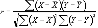 , (6.8)
and has a value of 1 for perfect correlation, a value of zero for no correlation, and a value of -1 for perfect anti-correlation.
The choice of an appropriate reference waveform is vital for the success of this technique in finding activations. The first approximation might be a square wave, which is high for scans acquired during the task, and low for scans acquired during rest (Figure 6.8a). Such a waveform however takes no account of the delay and smoothness of the haemodynamic response which regulates the BOLD contrast. An improvement to this would be to change the phase of the square wave (Figure 6.8b), with the delay being between 3 and 6 seconds.
To improve the reference waveform further, it is necessary to look more closely at the actual haemodynamic response. In an experiment such as the one used for the example data set, where there is both visual and motor activation, it is possible to use the response to one type of stimulus to form the reference waveform for finding the other. In this case the time series for one or more pixels in, say the visual cortex is extracted (Figure 6.8c), and correlation coefficients are calculated between this waveform and that of every other pixel in the image. Such an analysis detects only those regions in the brain which respond to the stimulus in the same way as the visual cortex. The major disadvantage of this technique is that it is particularly sensitive to motion artefact, since if such artefact is present in the reference waveform then the movement of other regions will be highly correlated. To attempt to reduce this, the response in the visual cortex to each stimulus can be averaged together, producing a mean response to the single cycle. The reference waveform is then made up of a repetition of these single cycle average responses (Figure 6.8d).
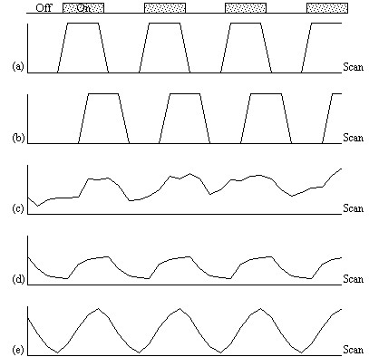
To be more general in predicting the haemodynamic response, so that a reference waveform can be constructed for any length of stimulus, it is necessary to know the response to a single stimulus. Friston[13] suggested that a haemodynamic response function could be considered as a point spread function, which smoothes and shifts the input function. By deconvolving the response from a known area of activation with the stimulus function, the haemodynamic response function can be obtained. The haemodynamic response function is not completely uniform across the entire brain however, and the shape obtained from one region may not be optimum for another. As an alternative, the response can be modelled by a mathematical function, such as a Poisson or beta function. The Poisson function
 (6.9)
(6.9)
with width l = 6 seconds, seems to fit well to observed haemodynamic responses (Figure 6.8e).
Since in general each slice of the volume imaged is not acquired at the same instant, it is necessary to accommodate timing differences in the correlation with the reference waveform. In order to do this, the relative magnitude of the activation at the time each slice was acquired is predicted, by convolving the input stimulus with a Poisson function. Then from this series, the correlation coefficients can be calculated on a slice by slice basis, constructing the reference waveform from the appropriate points in the predicted time series.
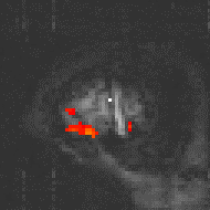
Examples of the effect of the reference waveform on the result is shown in Figure 6.9. Here, pixels in the head which correlate to the reference waveforms (shown in Figure 6.8), with r > 0.20 are shown in red, on top of the base image. The square wave correlation is the least effective in detecting activations (a), however a considerable improvement is obtained by delaying the waveform by 4 seconds (b). The correlation of the visual cortex with itself (c) is, not surprisingly, high, but using the average visual cortex response (d) improves the correlation in the motor cortex. The Poisson function model of the haemodynamic response (e) improves slightly on the delayed square wave, and is a good model.
|
|
(a) Square wave |
|
|
(b) Delayed Square Wave |
|
|
(c) Visual Cortex Response |
|
|
(d) Average Visual Cortex Response |

|
|
(e) Poisson Distribution Model |
The statistical techniques described above are both parametric tests. That is to say, they assume that the observations are taken from normal populations. Most parametric modelling techniques are special cases of the general linear model. This framework for analysing functional imaging data, first developed for PET and then extended for fMRI, is implemented in the software package SPM[14]. The general linear model is only outlined here, since the theory is extensively covered in the literature[15].
The aim of the general linear model is to explain the variation of the time course y1...yi...yn, in terms of a linear combination of explanatory variables and an error term. For a simple model with only one explanatory variable x1...xi...xn, the general linear model can be written
 (6.10)
where b is the scaling, or slope parameter, and ei is the error term. If the model includes more variables it is convenient to write the general linear model in matrix form
 , (6.11)
where now Y is the vector of observed pixel values, b is the vector of parameters and e is the vector of error terms. The matrix X is known as the design matrix. It has one row for every time point in the original data, and one column for every explanatory variable in the model. In analysing an fMRI experiment, the columns of X contain vectors corresponding to the 'on' and 'off' elements of the stimulus presented. By finding the magnitude of the parameter in b corresponding to these vectors, the presence or absence of activation can be detected.
b can be determined by solving the 'normal equations'
 (6.12)
where  is the best linear
estimate of b. Provided that (XTX)
is invertible then is given
by
is the best linear
estimate of b. Provided that (XTX)
is invertible then is given
by
 . (6.13)
Such parameter estimates are normally distributed, and since the error term can be determined, statistical inference can be made as to whether the b parameter corresponding to the model of an activation response is significantly different from the null hypothesis.
The general linear model provides a framework for most kinds of modelling of the data, and can eliminate effects that may confound the analysis, such as drift or respiration, provided that they can be modelled.
All the techniques described above require the prediction of the time course that active regions will follow. For many experiments, the use of rapid imaging, and carefully designed paradigms, makes the separation of the order of cognitive events possible. One such example, which is part of our study of Parkinson's disease and described in more detail in Chapter 7, is a paradigm involving the initiation of movement. In this experiment, the subject was required to respond, by pressing a hand held button, to the visual presentation of the number '5', and to make no response to the presentation of a '2'. This paradigm presented two differences to conventional, epoch based experiments. Firstly, the activations of interest, which are those responsible for the button pressing, occurred at an irregular rate. Secondly, all the cognitive processes involved in the task, including both the planning and execution of the movement, occurred in a time period of a few hundred milliseconds, as opposed to the sustained activation used in epoch based paradigms. Such an experiment requires a new form of analysis. Two techniques have been evaluated, both of which make no assumptions about the time course of activations during the task: the serial t-test, described here, and an analysis of variance technique, explained in the next section.
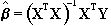
The basis of the serial t-test is to define a resting state baseline, and compare the images acquired at each time point before, during and after the task with this baseline. Figure 6.10 illustrates the technique. For each time point following the stimulus, a mean and standard deviation image is constructed, as is a baseline mean and standard deviation image. Then a set of t-statistical parametric maps are formed by calculating, on a pixel by pixel basis, the t-score (using equations 6.5 - 6.7) for the difference between mean image one and the mean baseline image, mean image two and baseline, and so on.
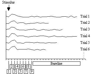
Figure 6.11 shows the result of analysing the example data set using this technique. Such a data set does not really show the benefit of the serial t-test analysis. Results shown in Chapter 7 better illustrate its use in looking at event timings, and unpredictable waveforms.
The technique has two major disadvantages. The first is that, in order to achieve a sufficient signal to noise ratio, it is necessary to have many more cycles than in an epoch based paradigm, thus leading to longer experiments. This can be uncomfortable for the subject, and puts additional demands on the scanner hardware. There is some scope for bringing the single event tasks closer together, but there must be a sufficient interval to allow the BOLD signal to return to baseline. This delay is at least ten seconds in length. The second disadvantage is that the analysis results in many statistical parametric maps, which have to be interpreted as a whole. However the fact that the technique makes few assumptions about the data time course makes it a strong technique, and opens up the possibility of more diverse experimental design, and a move away from the epoch based paradigms.
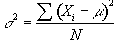
A second technique which does not require any assumptions about the shape of the activation time course, looks at the changes in variance upon averaging. The technique is based on simple signal averaging theory[16]. Take, for example, the response measured to a repeated signal as shown in Figure 6.12. The time series contains two components, one is a genuine response to the signal, and the other is the random fluctuations due to uncorrelated physiological events and noise in the image. Upon averaging 32 cycles together, the magnitude of the noisy component is reduced but that of the repeated signal is not. The reduction of the noisy component can be measured by calculating the variance of both the unaveraged and averaged data set.
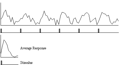
To detect regions of activation, the ratio of the variance of the averaged data set to the variance of the unaveraged data set is calculated for each pixel in the image. For pixels in regions of purely random intensity variations, this ratio will be around 1/n, where n is the number of cycles averaged together. Pixels in regions of activation, however, will have a significantly higher ratio than this, since the variance of both unaveraged and averaged data sets is dominated by the stimulus locked intensity variations of the BOLD effect, which does not reduce upon averaging.
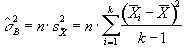
The technique is more formally explained as an analysis of variance (ANOVA)[17]. If Xij refers to the ith time point after the stimulus, of the jth cycle of an experiment
| time t | X11, | X12, | ....., | X1j, | ....., | X1n | X1 |
| time 2t | X21, | X22, | ....., | X2j, | ....., | X2n | X2 |
| ........ | ..... | ..... | ..... | ..... | ..... | ..... | ..... |
| time it | Xi1, | Xi2, | ....., | Xij, | ....., | Xin | Xi |
| ........ | ..... | ..... | ..... | ..... | ..... | ..... | ..... |
| time kt | Xk1, | Xk2, | ....., | Xkj, | ....., | Xkn | Xk |
| X |
with n cycles and k points per cycle. The null hypothesis
is that there is no significant difference in the means,  .
This can be tested by comparing two estimates of the population variance,
s2, one based on variations in measurements of the
same time point, and one based on the variance between time points.
.
This can be tested by comparing two estimates of the population variance,
s2, one based on variations in measurements of the
same time point, and one based on the variance between time points.
The variance within measurement of any time point can be calculated by
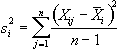 , (6.14)
and so the mean variance within time points is given by
 , (6.15)
and is based on k(n-1) degrees of freedom. The variance of the time point means is given by
 , (6.16)
and since
 (6.17)
then s2 can be estimated by
 (6.18)
which is based on k-1 degrees of freedom. Under the null hypothesis,
both  and
and  independently
estimate the population variance s2. This means that
the ratio
independently
estimate the population variance s2. This means that
the ratio
 (6.19)
will have an F distribution with k-1 and k(n-1)
degrees of freedom. If there is any signal change that is time locked to
the stimulus, the value of will
be larger than expected under the null hypothesis.
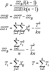
In the analysis of fMRI data, equations 6.15 - 6.19 are used to form an F-statistical parametric map. These equations are implemented using the following short-cut formulas
 (6.20)
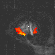
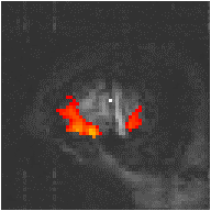
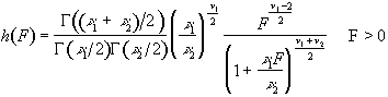
To assess the validity of this approach on real data, phantom and head images were analysed. The phantom data set consisted of 256 volume images, each of 128 x 128 x 16 matrix size, obtained at a repetition rate of 4 seconds. The head data set consisted of 256 head images, of the same matrix size, with the subject performing no specified task. Both data sets were pre-processed in the same way that a functional imaging data set would be, and the analysis of variance was then carried out assuming 16 points per cycle and 16 cycles. Histograms of F for each data set are shown in Figure 6.13, with the appropriate F distribution, shown as a dotted line, given by
 (6.21)
where n1 is the number of points per cycle minus one, and n2 is the total number of data points minus the number of points per cycle[18]. All three histograms show a good fit to the F distribution, confirming the validity of applying this technique to fMRI data.
| (a) | 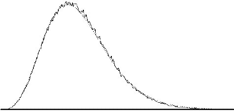 |
| (b) | 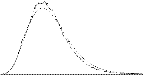 |
| (c) | 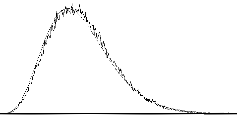 |
The results of analysing the example activation data set using the ANOVA technique are shown in Figure 6.14. As with the serial t-test, such a data set does not best show the potential of this technique. A better example comes from the analysis of a study to investigate short term memory.
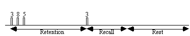
The stimulus paradigm for this experiment had three stages. First three digits in succession were presented to the subject. Eight seconds later a fourth digit was presented, and the subject was required to respond by pressing a button in their right hand if this final digit was the same as any of the three previously presented, or by pressing the button in their left hand if not[19]. The final stage was a period of rest, to provide a baseline. The whole test was repeated 32 times.
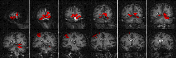
It would be expected that some regions of the brain would only be active during the presentation of the digits, some during the retention period, some only in the recall stage and others throughout the whole memory task. To analyse such data using a correlation technique would mean predicting a whole set of reference waveforms. The ANOVA technique, however, detected the responses of different shapes in one test. Figure 6.15 shows the activation maps obtained from the ANOVA analysis of the short term memory experiment, together with time course plots from several of the areas.
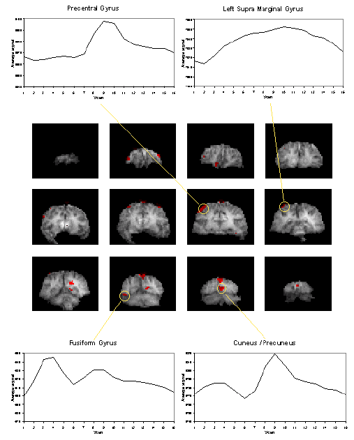
The final image of an ANOVA analysis, essentially shows all the regions which vary in some way that is synchronous to the presentation of the stimulus. It is equally good at picking up deactivations as activations. This makes these images a good starting point for other forms of analysis, such as principal component analysis or cluster analysis, so as to glean all the information that is available.
Due to the diversity of tests that can be carried out on one data set, software for implementing the tests described above was written as a set of separate programs.
The program correlate constructs a reference waveform, from user specified values, and optionally convolves this with a Poisson function of user specified width. Correlation coefficients are calculated using equation 6.8. If the reference waveform is made to vary between 0 and 1 then a measure of the percentage change upon activation can be obtained by calculating a linear regression of the form

where
 (6.22)
and
 .
.
The percentage change can be calculated as (b/a) x 100%.
The software also calculates the appropriate image of z-scores using Fishers Z transform and the reduced degrees of freedom as explained in the following sections. The file names for each of these outputs is
| cc_<file>.img | correlation coefficients saved as 'shorts' x 10,000 |
| pc_<file>.img | percentage change saved as 'shorts' x 1,000 (such that 1% signal change x 1,000) |
| cz_<file>.img | z-scores saved as 'floats' (not scaled) |
The serial t-tests are performed by tmap and tmapnc, the first appropriate for cyclic experiments and the second for non-cyclic experiments. For the non-cyclic version the stimulus times are obtained from a text file, and both output t-score maps saved as 'shorts', scaled by 1000, in a file named tt_<file>.img.
ANOVA tests are carried out by the programs anova, and anovanc, which both output f-scores scaled by 1000, in a file named va_<file>.img.
The statistical analysis techniques discussed in the last section all result in a statistical parametric map (SPM), where each pixel in the image is assigned a value based on the likelihood that the null hypothesis is false. However for the localisation and comparison of brain function, what is required is an image which only highlights those pixels which can confidently be labelled as active. This is done by thresholding the statistical parametric map.
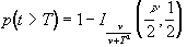
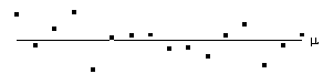
Before approaching the problem of the significance of whole images, it is necessary to consider the question of the confidence that can be placed in the result of a single t-test, correlation or ANOVA. Such levels come from an understanding of the distribution, under the null hypothesis, of the statistic being considered. If for example a statistic had a normal distribution, as shown in Figure 6.16, a critical value Za can be defined such that
 . (6.23)
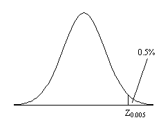
This means that if the value of Z obtained in the statistical calculation is greater than Z0.005, we can be 99.5% confident the null hypothesis is false. The number 0.005 in such a case is said to be the p-value for that particular test. Such values are tabulated in standard statistical texts, or can be obtained directly from expressions for the distributions themselves.
The distribution for a correlation coefficient is dependent on the number of degrees of freedom in the time course being analysed. For a time course of n independent time points, there are n-2 degrees of freedom. The question of whether time points from an fMRI experiment are independent is addressed later in this section. The correlation coefficient, r, can be transformed so that it has a Z distribution (that is a Gaussian distribution with zero mean and unit variance), by applying the Fisher Z transform
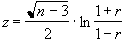 . (6.24)
This transform may therefore be applied to the SPM of correlation coefficients, yielding an SPM of z scores.
The theory of Gaussian random fields (as described later, in section 6.4.3), applies to images of z scores. Therefore it is necessary to transform the t and f scores to z scores as well. This is done by calculating the area under the distribution (p value) between t and infinity (or f and infinity), and choosing an appropriate value of z such that the area under the Z distribution between z and infinity is the same.
P-values for the t-statistic are related to the incomplete beta function
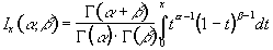 (6.25)
such that
 (6.26)
where n is the number of degrees of freedom, which is equal to the number of data points that were used to construct the statistic minus one.
Similarly p-values for the f-statistic can be derived from
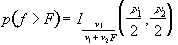 (6.27)
where n1 is the number of points per cycles minus one and n2 is the total number of points minus the number of points per cycle (n1=k-1, n2=k(n-1)).
The transforms are carried out using pre defined functions in the package MATLAB[20], to calculate the incomplete beta function and the inverse error function.
All the statistical tests assume that the data points are independent samples of the underlying population. This however may not be the case, since the effect of the haemodynamic response function, and any temporal smoothing that is applied to the data, means that adjacent time points are no longer independent. This has an effect on the effective number of degrees of freedom in the sample.
A detailed analysis of this problem is given in by Friston et. al.[21-23], but a more intuitive explanation of his result is given here.
Consider a series of n independent observations of a population of mean m.
The variance of the population is given by
 (6.28)
which is best estimated by the sample variance
 . (6.29)
The denominator in this expression is the number of degrees of freedom of the sample, and is one less than the number of observations, since only n-1 points are needed to describe the sample, the 'last' point being determined by the mean.
Now if the above data set is smoothed with a three point running filter such that
 .
.
The sum of the square deviations from the mean of the data is now (on average) three times less than that of the unsmoothed data. This means that the population variance is now best approximated by
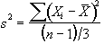 (6.30)
and implying that the smoothed data set has (n-1)/3 degrees of freedom. In the case of the pre-processing described above, the smoothing filter is a Gaussian kernel, as opposed to the three point running average.
In this case it is necessary to evaluate the effect of neighbouring data points on any one point, and so the reduction in the number of degrees of freedom is given by the area under the Gaussian kernel. The number of degrees of freedom in the sample variance for a data set of n sample points, smoothed with a Gaussian of standard deviation s is therefore
 . (6.31)
Simulations of the effect of smoothing data before carrying out an analysis of variance calculation show that such a degrees of freedom reduction does not hold in this case. Temporal smoothing of the data is unlikely to improve the ability of the ANOVA test to detect activations, and is therefore best not applied, however high pass filtering is likely to improve the test and should still be used.
A summary of the number of degrees of freedom for the tests described earlier is given below.
All the reasoning so far in this section is to do with the p values concerned with one statistical test. That is to say, for one individual pixel, we can be confident to a certain value of p, that its time course is correlated to the stimulus. When we form an image from the results of such statistical tests, it is necessary to consider how confident we are that none of the pixel labelled as 'active', are in fact due to random fluctuations. Take for example the SPM shown in Figure 6.17.
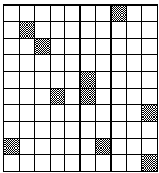
Here a pixel is shaded if a statistical test shows that the pixel is active, with a p value greater than 0.1. Since there are 100 pixels in the image, it is probable that 10 pixels will, by chance, be falsely labelled as active. The p value for such an image would therefore be 1.0, that is to say that we are certain that at least one of the pixels is falsely labelled. This situation is called the multiple comparisons problem, and is well studied in statistics[24].
If all the pixels can be considered to be independent, then a Bonferroni correction can be applied. This states that for an image of N pixels, the overall probability of any false positive result is P, if the individual pixel false positive probability is P/N. However with thousands of pixels in an image, such a technique is very stringent, and the risk of falsely rejecting true activations is very high. There is also the question of whether each pixel in the image can truly be regarded as independent. The point spread function of the imaging process means that adjacent pixels cannot vary independently, and this situation is worse if additional smoothing is applied.
Such problems were first addressed in PET data analysis, and the results carried over to fMRI. The theory of Gaussian random fields[25], was developed for the analysis of functional imaging data by Friston et. al.[26] and an overview of their important results is presented here.
For a completely random, D-dimensional, z-statistical parametric map consisting of S pixels, the expected number of pixels that are greater than a particular z score threshold, u, is given by
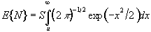 . (6.32)
This is the area under the Gaussian distribution as shown in Figure 6.16. The theory attempts to estimate the number of discrete regions there will be above this threshold. Take for example the SPM shown in Figure 6.18a. This is formed from a simulated data set with completely independent pixels. Those pixels with z-scores above a certain threshold are shown in white with those lower in black. The same data set, spatially smoothed before analysis is shown in Figure 6.18b. The number of white pixels in each SPM is about the same, but the number of discrete regions of white pixels is much less in the smooth case.
(a)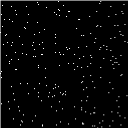 (b)
(b)
The expected number of regions appearing above u is estimated by
 (6.33)
where W is a measure of the 'smoothness', or resolution of the map. This is obtained by measuring the variance of the first derivative of the SPM along each of the dimensions
 . (6.34)
The average size of a region is thus given by
 . (6.35)
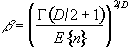
Once these quantities have been estimated, the question is, what is the probability that a region (of activation) above a certain threshold u of size k pixels, could occur purely by chance. If k is of the order of E{n} then this probability is quite high, but if k»E{n} then the probability reduces. The form of this probability distribution is taken as
 (6.36)
where nmax is the size of the maximum region above u, in a random SPM, and
 . (6.37)
Thus for a given SPM the smoothness parameter W can be calculated, and only those regions above a chosen value of u that are of size greater than a chosen k are shown, the p value for the activation image can be calculated using equations 6.32 - 6.37.
Having thresholded the SPM to display only those 'active' regions, these regions must be superimposed on background images to enable anatomical localisation. If the EPI images that the fMRI data comes from are of suitable quality, then these can be used as the base images. Better contrast may come from some inversion recovery images (see Section 2.4.1) showing only white matter, or grey matter. This is the practice used for the images shown in Chapter 7, and has the advantage that any distortions in the images will be the same for both activation and background, and no image realignment is needed. Higher resolution EPI images with equal distortion can be obtained using interleaved EPI as discussed in Chapter 5. To obtain really high quality base images it is necessary to use a 2DFT technique, however the distortions in such an image will be much less than the EPI functional images, and some form of alignment and 'warping' is required in this case.
The subject of comparing results from a number of different experiments, either on the same person at different times, or between different people, raises many issues, only a few of which are covered here.
Qualitative comparisons between subjects can be made by a good radiologist, familiar with EPI images, however in order to quantify differences it is necessary to try and 'normalise' the differences between the brains of the subjects. This has traditionally been done in functional imaging by using the atlas of Talairach and Tournoux[27], based on slices from the brain of a single person. It uses a proportional grid system based on the location of two anatomical landmarks, the Anterior Commissure (AC) and the Posterior Commissure (PC). Having identified the locations of the AC, PC, and the superior, inferior, left, right, anterior and posterior edges of the brain, these co-ordinates are rotated until the line joining the AC and PC is along the x axis, and the line joining the left and right markers is parallel to the z axis (Figure 6.19).
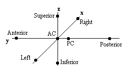
The same rotations are performed on any 'activation' region, and the co-ordinates are then scaled to give a distance in millimetres from the AC in each dimension, such that
These readings can then be looked up in the atlas to determine the location of the activation. Alternatively the whole image set can be similarly transformed to give a Talairach normalised set of images.
The main drawback of this technique is that it is based only on the brain of one person, and since gyri and sulci vary significantly between people, the reliability of using such an atlas is questionable. It is also questionable as to whether the proportional grid system is reliable enough to transform the images. As an alternative it is possible to warp the image until it fits the Talairach atlas brain[28]. If warping is used, then there are more appropriate templates available, which are based on MRI scans of a number of subjects. These templates attach probabilities to the spatial distribution of the anatomy[29], and are more reliable than a single subject template.
Even if the brains of several subjects are in some way normalised, there are questions as to how significant are differences in the magnitude of the signal change from one subject to another. A large amount of subject movement during the scanning will reduce the statistical likelihood of detecting activations. This could mean that activation which is present, but not detectable due to poor signal to noise, could be interpreted as no activation at all. Such problems have no easy solution, and more work is required in this area.
Consideration of these problems for a specific experiment is given in Chapter 7.
Software was written which allowed the user to interactively change the values of u and k, and to look at the effect that this has on the activation image and its p-value. The graphical user interface (shown in Figure 6.20) is written in the scripting language 'perl'[30], which calls other 'C' programs to carry out most of the calculations and data manipulation.
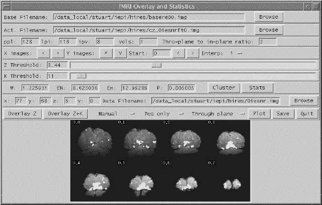
SPMs of z-scores, stored as floats, are read in and thresholded at a z-score specified by a slider. These are displayed as white pixels, above a greyscale base image. The user can choose an appropriate cluster size threshold by either changing the slider or clicking on one of the regions with the mouse, and asking for the calculation of the size of that cluster. The activation image, with both thresholds applied can be displayed, and the p-value for such a combination calculated. It is necessary to change both thresholds interactively to find the optimum activation image for a given p-value, however results from Friston[31] suggest that wide signals are best detected using low z-thresholds and sharp signals with high z-thresholds.
The time course plots for any selected region can be displayed, with the 'plot' option. Any file can be chosen to take the plot intensities from, allowing the whole experiment time course, the average for one cycle, or Fourier components for the region to be displayed, provided that an image file containing such data exists.
Having chosen an appropriate set of thresholds, the images can be saved for display. The 'save' option allows any image file to be overlaid upon the base file, masked by the thresholded SPM. The base images are scaled between 0 and 20,000, and the 'active' regions scaled between 20,000 and 32,000, which allows an appropriate image viewing package to display the base images in greyscale and the activation in colour-scale. If the statistic used is also a good indicator of the magnitude of activation signal change, for example the t-statistic for the difference between 'rest' and activity, then it is appropriate to display in colour-scale the pixel values from the SPM. However for statistics such as the correlation coefficient, the values do not represent the amount of signal change. In these cases it is more appropriate to display values from a percentage change image in colour, masked by the thresholded SPM. In order to appropriately identify the anatomical location of the activation, it is sometimes desirable to see the brain structure that underlies the activation. In this case it is appropriate to use the base images as the source of the values for the activation regions. This means that the effect can be created where the background image is in greyscale, and the active regions are 'shaded' in red-scale. Examples of overlaying SPMs, regressions and base sets are shown in Figure 6.21.
| (a) | 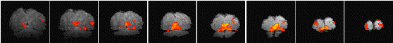 |
| (b) |  |
| (c) | 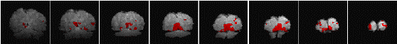 |
The software can also calculate the Talairach co-ordinates of any region, provided that the appropriate landmarks can be identified (or deduced) from the images. Having entered the co-ordinates of the landmarks, and chosen a region of interest, the co-ordinate system is rotated and proportionated, to give the distances in millimetres from the Anterior Commissure, of the centre of mass of that region in Talairach space.
The user instructions for the software is included as Appendix C.
The most important aspects of fMRI data analysis, as used on the data in this thesis have been presented above. The pre-processing steps improve the ability of the statistical analysis to detect activations. The choice of an appropriate statistical test depends on the assumptions that can be reasonably made, and the questions that need to be addressed. Decisions about the statistical significance of the results must take into account the multiple comparisons problem, and the reduction in degrees of freedom resulting from smoothing. Finally the results must be presented in an appropriate form, to enable the comparison of results between subjects.
In the whole process, many informed decisions need to be made, and it is difficult to propose a single 'black box' approach to the analysis, where data is fed in and an activation image is automatically fed out. However in order to formalise the analysis procedure to some degree, a standard analysis protocol was written. This is included as Appendix D.
There are many more issues in the analysis that have not been mentioned here, and much work that can be done. For example the Fourier Analysis methods for detecting periodic activations[32] , principal component analysis[33], clustering techniques which detect clump together pixels having time courses which vary in the same way, and nonparametric tests[34]. There are other methods for solving the multiple comparison problem [35] and for carrying out inter subject comparisons. It is this last area which requires the most attention, since, as fMRI becomes more and more a tool for neurologists to detect abnormality in brain function, the reliability of inter subject comparisons will become more important. It has been well shown that fMRI can give colourful pictures of the brain working, and it is necessary to take the techniques for data analysis onward if fMRI is to fulfil its clinical and neurological research potential.
[1]four1() from Press, W. H., Teukolsky, S. A., Vetterling, W. T. and Flannery B. P. (1992) `Numerical Recipes in C', Cambridge University Press.
[2] The motion correction software described was written by Dr. A. Martel, Department of Medical Physics, University of Nottingham.
[3] Hu, X., Le, T. H., Parrish, T. and Erhard, P. (1995) Retrospective Estimation and Correction of Physiological Fluctuation in Functional MRI. Magn. Reson. Med. 34,201-212.
[4] Friston, K. J., Williams, S., Howard, R., Frackowiak, R. S. J and Turner, R. (1996) Movement-Related Effects in fMRI Time-Series. Magn. Reson. Med. 35,346-355.
[5] Oppenheim, A. V. (1978) `Applications of Digital Signal Processing', Prentice Hall.
[6] Friston, K. J., Holmes, A. P., Poline, J.-B., Grasby, P. J., Williams, S. C. R., Frackowiak, R. S. J. and Turner, R. (1995) Analysis of fMRI Time-Series Revisited. Neuroimage 2,45-53.
[7] See Kernighan, B. W. and Ritchie, D. M. (1978) `The C Programming Language', Prentice-Hall.
[8] Analyze. Biomedical Imaging Resource, Mayo Foundation.
[9] Bandettini, P. A, Jesmanowicz, A., Wong, E. C. and Hyde, J. S. (1993) Processing Strategies for Time-Course Data Sets in Functional MRI of the Human Brain. Magn. Reson. Med. 30,161-173.
[10] SPM from the Wellcome Department of Cognitive Neurology http://www.fil.ion.ucl.ac.uk/SPM.
[11] Zar, J. H. (1996) `Biostatistical Analysis', Prentice-Hall.
[12] Miller, I. and Freund, J. E. (1977) `Probability and Statistics for Engineers', Prentice-Hall.
[13] Friston, K. J., Jezzard, P. and Turner, R. (1994) Analysis of Functional MRI Time-Series. Human Brain Mapping 1,153-171.
[14] SPM from the Wellcome Department of Cognitive Neurology http://www.fil.ion.ucl.ac.uk/SPM.
[15] Friston, K. J., Holmes, A. P., Worsley, K. J., Poline, J.-B., Frith, C. D. and Frackowiak, R. S. J. (1995) Statistical Parametric Maps in Functional Imaging - A General Linear Approach. Human Brain Mapping 2,189-210.
[16]Lynn, P. A. (1989) `An Introduction to the Analysis and Processing of Signals'. Macmillan.
[17] Guenther, W. C. (1964) `Analysis of Variance'. Prentice-Hall.
[18] Mood, A. M. and Graybill, F. A. (1963) `Introduction to the Theory of Statistics'. McGraw-Hill, Second Edition p232.
[19] Hykin, J., Clare, S., Bowtell, R. Humberstone, M., Coxon, R., Worthington, B., Blumhardt, L. D. and Morris, P. A Non-directed Method in the Analysis of Functional Magnetic Resonance Imaging (fMRI) and it's Application to Studies of Short Term Memory in Book of Abstracts, 13th Annual Meeting, European Society of Magnetic Resonance in Medicine and Biology 366.
[20] MATLAB. The Math Works, Inc.
[21] Friston, K. J., Jezzard, P. and Turner, R. (1994) Analysis of Functional MRI Time-Series Human Brain Mapping 1,153-171.
[22] Friston, K. J., Holmes, A. P., Poline, J.-B., Grasby, P. J., Williams, S. C. R., Frackowiak, R. S. J. and Turner, R. (1995) Analysis of fMRI Time-Series Revisited Neuroimage 2,45-53.
[23] Worsley, K. J. and Friston, K. J. (1995) Analysis of fMRI Time-Series Revisited - Again Neuroimage 2,173-181.
[24] Zar, J. H. (1996) `Biostatistical Analysis', Prentice-Hall. p.211.
[25] Cox, D. R. and Miller, H. D. (1990) `The Theory of Stochastic Processes', Chapman and Hall.
[26] Friston, K. J., Frith, C. D., Liddle, P. F. and Frackowiak, R. S. J. (1991) Comparing functional (PET) images: The assessment of significant change. J. Cereb. Blood Flow Metab. 11,690-699.
[27] Talairach, J. and Tournoux, P. (1988) `Co-planar Stereotaxic Atlas of the Human Brain', Thieme.
[28] Collins, D. L., Neelin, P., Peters, T. M. and Evans, A. C. (1994) Automatic 3D Intersubject Registration of MR Volumetric Data in Standardized Talairach Space. J. Comput. Assist. Tomogr. 18,192-205.
[29] Mazziotta, J. C., Toga, A. W., Evans, A., Fox, P. and Lancaster, J. (1995) A Probabilistic Atlas of the Human Brain: Theory and Rationale for its Development. Neuroimage 2,89-101.
[30] See Wall, L. and Schwartz, R. L. `Programming Perl', O'Reilly & Associates.
[31] Friston, K. J., Worsley, K. J., Frackowiak, R. S. J., Mazziotta, J. C. and Evans, A. C. (1994) Assessing the Significance of Focal Activations Using their Spatial Extent Human Brain Mapping 1,214-220.
[32] Lange, N. and Zeger, S. L. (1997) Non-linear Fourier Time Series Analysis for Human Brain Mapping by Functional Magnetic Resonance Imaging. Applied Statist. 46,1-29.
[33] Backfrieder, W., Baumgartner, R., Sámal, M., Moser, E. and Bergmann, H. (1996) Quantification of Intensity Variations in Functional MR Images Using Rotated Principal Components. Phys. Med. Biol. 41,1425-1438.
[34] Holmes, A. P., Blair, R. C., Watson, J. D. G. and Ford, I. (1996) Nonparametric Analysis of Statistic Images from Functional Mapping Experiments. J. Cereb. Blood Flow Metab. 16,7-22.
[35] Forman, S. D, Cohen, J. D., Fitzgerald, M., Eddy, W. F., Mintun, M. A. and Noll, D. C. (1995) Improved Assessment of Significant Activation in Functional Magnetic Resonance Imaging (fMRI): Use of a Cluster-Size Threshold. Magn. Reson. Med. 33,636-647.