For each region of the brain, or cognitive paradigm that is to be studied with MRI there are specific issues regarding the optimisation of the fMRI experiment. These are covered in the chapter on functional MRI applications. There are however issues that relate more generally to fMRI experiments, such as dealing with artefacts and the optimisation of echo time. These subjects are covered here.
The first section deals with the effect of echo time on the magnitude of the signal detected as a result of the BOLD effect. A single shot technique for obtaining images with different echo times is described, and this is also used to produce T2* maps during brain activation. Next, two artefact reducing methods are discussed. The first to reduce the N/2 ghost, and the other to remove artefact from external r.f. interference. A pulse sequence which reduces the time taken to acquire inversion recovery anatomical reference scans is presented, and in the final section the rationale behind a standard experimental protocol for fMRI experiments is explained.
As was described in Chapter 3, task performance causes a local increase in the value of T2* in the region of the brain that is involved in the task, which can be detected in T2* weighted images. The amount of T2* weighting that is seen in an image depends on the echo time, TE (see section 2.4.2). For a given value of T2*, images obtained with a value of TE equal to T2* will be optimal at detecting any change in T2* (see section 3.3.3). The magnitude of T2* depends on a number of factors that are scanner dependent, such as field strength and quality of shimming, and others that are object dependent, such as the orientation of the boundaries between regions with differing magnetic susceptibility.
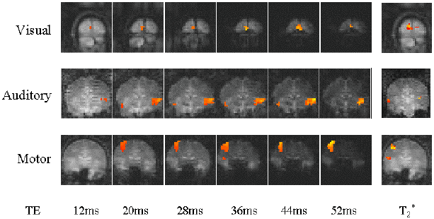
Given this, it becomes important to find the value of TE which will give the best detection of even the smallest changes in T2* in the region of brain that is being studied. This has been done previously by carrying out several experiments, each using different echo times [1]. Changes in the value of T2* upon visual activation have also been measured using spectroscopy [2], and multi echo FLASH [3]. More recently, a double echo time approach to T2* mapping has been demonstrated [4]. Here, a technique is presented which obtains a set of low resolution images with six different echo times from a single FID. This enables activation images from each different echo time to be obtained for precisely the same task. By fitting T2* curves to the data, it has also been possible to obtain maps of T2* during activation. This sequence has been used in activation experiments involving visual and auditory stimulation, and motor tasks on five normal volunteers.
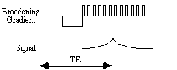
In EPI, a gradient echo is formed in the broadening direction by applying an initial dephasing gradient, and then a series of 'blips' of the opposite polarity which form the echo. The time from the r.f. excitation pulse to the centre of the echo is defined as the echo time in EPI (see Figure 4.1). This is distinct from the repeated set of echoes formed by the switching of the read gradient.
Having formed one gradient echo, it is possible to form other echoes simply by reversing the polarity of the blipped gradient. These echoes all form under the T2* decay envelope, and have different echo times (Figure 4.2). This is distinct from the multiple spin echo experiment described in section 2.4.3, in which the echoes form under the T2 decay envelope.

The signal can continually be recalled in this way, provided that T2* has not already reduced the signal to zero.
The above sequence was implemented on a dedicated EPI 3.0 Tesla scanner, with purpose built head gradient coils, birdcage r.f. coil, and control. In order to sample at 6 echo times between 10 and 55 ms, a matrix size of 32 x 32 and a switching rate of 1.9 kHz was chosen. This gave echo times of approximately 12, 20, 28, 36, 44 and 52 ms, and a voxel resolution of 5 x 5 x 10 mm3. The ordering of the rows in the 2nd, 4th and 6th echo time image was reversed prior to Fourier transformation to maintain the equivalent orientation of the images.
A T2* map was calculated for every FID by fitting the data from each echo time, on a pixel by pixel basis, to an exponential decay curve of the form
![]() .
.
(4.1)
This was done by taking the logarithm of the pixel intensity and calculating the linear regression, intercept and correlation coefficients between these and the echo time. These values were used to form images of T2*, S0 and correlation.
The activation experiments were designed to produce a response in the visual, motor and auditory cortices. For the visual and motor experiment, the subject observed an LED display. During the task condition, an outer ring of LED's lit, and a central bar flashed at a rate of 2 Hz. The subject was required to respond to the stimulus by pressing a hand held button at the same rate as the flashing LED. The whole brain was imaged, in 16 slices, every 4 seconds. The experiment consisted of 16 seconds of rest followed by 16 seconds of activity, repeated 32 times, and was carried out on 5 normal volunteers.
The auditory experiment consisted of imaging 6 slices through the temporal lobes in 600 ms, each set of slices being acquired every 14 seconds. In alternate gaps, a 14 second recording of speech was played to the subject. Thus for each cycle one volume set of images was obtained directly after a 14 second period of auditory stimulation, and one set was acquired after a 14 second period of silence. The advantage of carrying out the experiment in this way is that the auditory stimulation from the scanner does not interfere with the auditory stimulation of the speech. Each experiment consisted of 20 cycles of speech and silence, and was carried out on 5 normal volunteers.
The analysis of the data was carried out using the techniques and software described in Chapter 6. Following image formation, the echo time data was normalised, spatially filtered with a 3D Gaussian kernel with FWHM of 6 mm, and temporally filtered with a Gaussian kernel of FWHM 3 s. For the visual and motor experiment the time course was correlated to a delayed and smoothed reference waveform (square wave convolved with a Poisson function with l = 6 s), on a pixel by pixel basis to produce one statistical parametric map (SPM) for each echo time.
The auditory activation data was analysed using a t-test comparison between the mean of the speech and silence images, again forming one SPM for each echo time. The correlation coefficients and t-scores were transformed to z-scores and thresholded to the same p-value using both peak height and spatial extent of the SPM.
For each echo time, the mean percentage change between activation and rest was calculated, for all the pixels in the active regions. In order to ascertain which echo time yields the optimum results, the product of the mean percentage change and the number of pixels in the activated region was calculated.
Similar statistical analysis was performed on the T2* maps.
Examples of the activation images produced, for each echo time and for the T2* maps, are shown in Figure 4.3. The colours in the active regions refer to the level of percentage change in each region, and these are overlaid on the mean of the images acquired at that echo time. The levels of significance of the activation (p value) were less for the T2* maps than for the T2* weighted images, however discrete regions of activation in the same regions can be seen. The general trend is for the percentage change to increase with echo time, however the extent of the activation detected reduces with the longer echo times. This is illustrated in the graphs of the product of percentage change and number of active pixels, shown in Figure 4.4 for each of the subjects. The dotted line on these plots represents the activation from the T2* maps. The level of percentage change observed in the T2* maps upon activation was usually greater than that observed in the T2* weighted images, but the regions were generally smaller. No significant change was detected in the maps of S0 during the tasks.
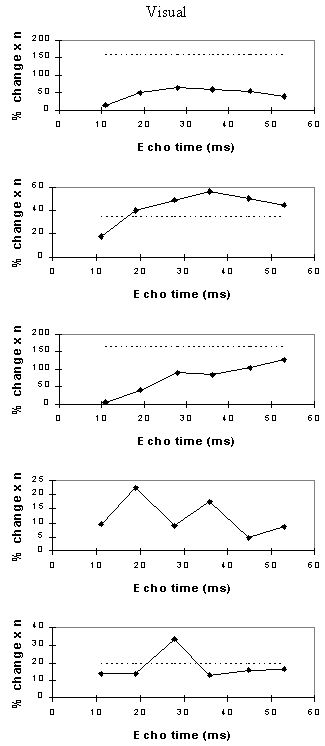
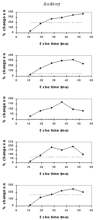
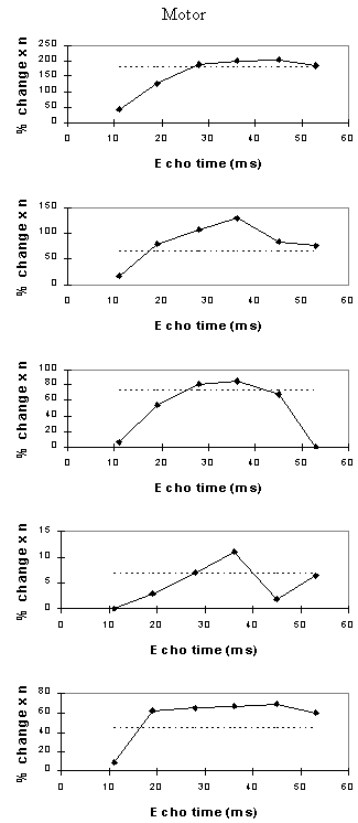
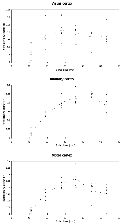
An appropriate choice of echo time for the motor and auditory cortices, would appear to be between 30 and 40 ms, and between 25 and 35 for the visual cortex. If the echo time is too short, the percentage change is so small that the activation response is lost in the contrast to noise of the time series. However if the echo time is too long, the signal from the cortex has fallen to zero due to T2* decay and no change is seen on activation.
The multiple gradient echo technique produces, from a single FID, a set of images with different values of echo time. Measuring several echo times in one experiment has the advantage of reducing the total experimental duration, and eliminating the effects that habituation, subject restlessness, or repositioning could have on the results if separate experiments were carried out at each echo time. The results suggest that an echo time of between 25 and 40 ms would be optimum for experiments in the visual, motor and auditory cortices at 3 T. More results would be required in order to be confident of using a similar echo time for studies in other regions of the brain, but this technique offers a quick and simple way to carry out such an experiment.
The relatively thick slices used, will mean that through slice dephasing will reduce the values of T2*. The slice thickness of 10 mm used in this experiment is comparable to that used in many whole brain studies, however the choice of optimum echo time may be different for the thinner slices used in some experiments.
The use of T2* maps, instead of T2* weighted images for fMRI has the additional benefit that the results will not be so affected by in-flow effects, or through slice movement artefact. If higher resolution images were required, the number of echo times recorded could be reduced, so that the number of lines in the image could be increased. For example four 64 x 64 images could be acquired with echo times of 16, 32, 48 and 64 ms, and T2* curves fitted to this data, allowing an in plane resolution of up to 3 mm.
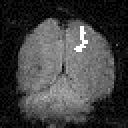
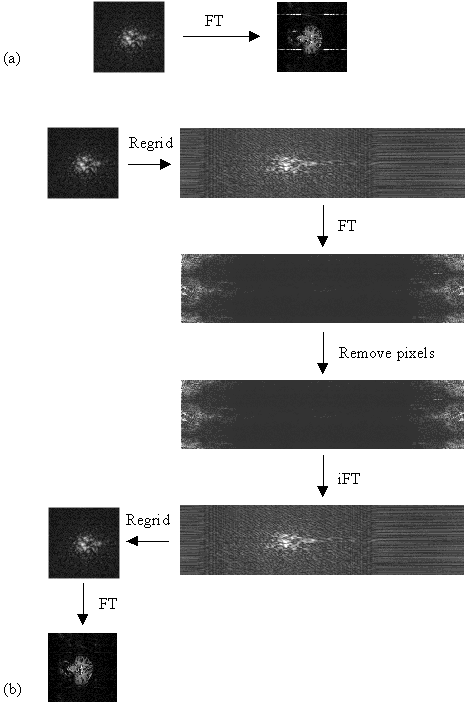
One type of artefact which is specific to EPI is the Nyquist, or N/2 ghost. This arises because odd and even echoes are acquired under opposite read gradients, and the data requires reversal prior to image reconstruction. Inaccurate timing of the sampling relative to the switched gradient, temporal asymmetries in the analogue filter or inhomogeneities in the static field cause a modulation of alternate lines in k-space. This leads to a ghost image shifted by N/2 pixels in the phase encode direction. An example of this effect is shown in Figure 4.5a, where the phase of alternate lines in k-space has been altered by a small amount. If the image and ghost overlap, interference occurs leading to fringes in the image as shown in Figure 4.5b.
(a)  (b)
(b) 
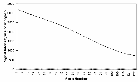
In fMRI, ghosting artefact can cause a number of problems. In the first place, the ghosting can spoil the look of the image, and ghosting of activated regions could lead to apparent 'activation' appearing outside the head. More serious effects occur if the artefact changes with time. Movement of the subjects head causes the interference fringes, of overlapping ghost and image, to change dramatically, with even small displacements having a large effect. Since subject motion is often stimulus correlated, particularly if the experimental paradigm involves movement, the changes of the interference pattern can show up in the statistical analysis as 'activation', as shown in Figure 4.6. It has also been observed on our scanner that the ghosting can change with time as shown in Figure 4.7, from an experiment lasting eight minutes. This probably results from changes in the switched gradient waveform as the coil heats up and its resistance increases.
The N/2 ghost can be reduced by making hardware improvements in filter performance and reducing eddy currents. There is however a limit to the technical improvements that can be made, so a number of techniques for correcting such artefact in post-processing have been proposed. These techniques are described in this section and are tested on phantom and head fMRI data sets to compare their usefulness in this application.
The simplest form of ghost reduction is to apply a phase angle correction to each point in alternate lines of the k-space data. The required phase correction can be determined by eye, and applied to every image in the fMRI data set. The effect of eddy currents can be modelled by an alternate echo phase variation in the read (x-) direction

(4.2)
so by applying a first order correction, ghosting from such effects can be reduced. A mismatch in the sampling can be corrected by a linear shift of the real and imaginary time data.
All these methods go some way towards removing the N/2 ghost, but will not remove ghosts caused by more complicated phase errors. The subject of N/2 ghosting is extensively covered in a paper by Bruder et. al. [5] in which a method based on a calibration scan is proposed. Such a scan is acquired with no broadening gradient so, in an ideal case, equivalent points in all the echoes would have the same phase. Bruder's method applies a phase correction to force each echo in the calibration scan to have the same phase, and then applies this same phase correction to the (broadened) image. So if the ith line of the calibration scan has phase qi(x) then the corresponding line in the image is phase corrected by an angle -qi(x) . This can be carried out practically on a time-point by time-point basis, without directly calculating the phase angles, using the formula
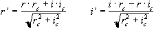 (4.3)
(4.3)
where r and i represent the real and imaginary components of the data point and the subscript c represents the calibration scan data.
An alternative form of calibration scan has been proposed by Hu [6]. In this case the reference scan consists of an image acquired under reversed switching gradients. That is to say, if the first line of the normal image is acquired under a positive read gradient, then the first line of the reference image is acquired under a negative read gradient. These two images could be spliced together, so that the final image is made up from only lines that were acquired under a positive read gradient, much in the way that EPI was first proposed [7]. However Hu proposed that the even lines of the reference scan be used to correct the odd lines of the actual image, so that a single reference scan can be used to phase correct a whole set of images. Initially all the lines of the normal images and the reference scan are Fourier transformed in the read direction. Next the even lines of the reference image are reversed. The phase correction q that must be applied to these lines in the corresponding normal image in order for them to have the same phase as the reference image is given by
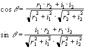
(4.4)
where the subscript 1 refers to the normal image and the subscript 2 refers to the reference image. This correction can then be applied to all the images using
(4.5)
again where r is the real component and i is the imaginary component of the complex data point. Finally the images are Fourier transformed along the phase encode direction to form the corrected image.
This technique can be further extended by collecting two reference scans, without the broadening gradient applied, one with a positive read gradient for the first echo and the other with a negative gradient. This has the advantage that there is more signal present in the earlier and later lines of k-space to enable a better calculation of the phase correction required in these lines.
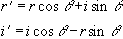
An alternative method that requires no reference scans has been proposed by Buonocore [8]. If two images are constructed, one from only the odd echoes, with the even echoes zero filled prior to Fourier transformation, and one from only the even echoes, with the odd echoes zero filled, then both images will display ghosting, one with a positive ghost, and one with a negative ghost (see Figure 4.8). If there were no phase errors in the odd and even echoes then the phase difference in the object only region (that is where there is no ghost) between these two images would be zero. However if there are phase errors, then a phase difference between equivalent points in the odd and even image of 2q(x,y) can be detected. If the ghost and image do not overlap, it is possible to add the two images together, having applied an appropriate phase correction to one, to form a ghost free image. However if they do overlap then the phase differences are calculated as a function of x only (that is along the read direction) and averaged through all the lines in the object only region as defined by the user. Having determined the phase difference, the original time data can be corrected by Fourier transformation in the read direction, multiplying the odd lines by exp(iq(x)) and the even lines by exp(-iq(x)).
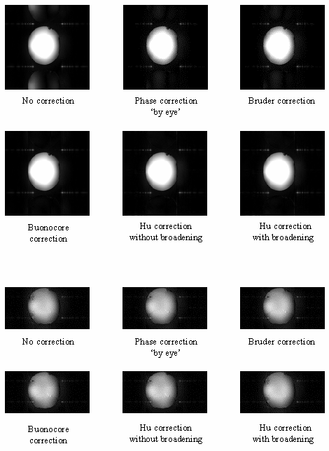
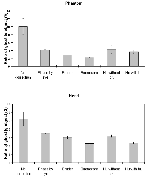
The above five methods were tested on both phantom and head data, with objects that fill and half-fill the field of view. Examples of their ability to correct the ghosting are shown in Figure 4.9a-b. Most of the corrections reduce the ghosting partially in the phantom images. Where the ghost and object overlap, the Hu correction with broadening is slightly better at reducing the ring the edge of the ghost.
To quantify the level of ghosting, regions of interest (ROI) were drawn around the object and the ghost region of the images in which the object half-filled the field of view. Six images of the same phantom, each with different levels of ghosting, were corrected using all five techniques. The mean intensity of the ghost as a percentage of the mean intensity of the object for each technique is shown in Figure 4.9c. The Hu correction without broadening, does not perform as well as might be expected. This is because of the complete failure of the technique in correcting the column in which the external r.f. interference appears, thus producing bright streaks in the ghost region. The Buonocore method appears in both cases to be the best method.
All the above techniques, apart form the Buonocore method, will not correct phase errors that change with time. Since changes in the ghost do occur with time, adaptations of the above techniques are needed if they are to deal with such situations. If ghost only and object only regions can be defined, as is the case if the object does not fill the field of view, then a zeroth or first order alternate line phase correction can be applied which minimises the signal in the ghost region relative to the object region. This technique can work very well in some cases, however if there is any overlap of image and ghost, then the minimisation can occasionally produce obviously incorrect results. Alternatively, the ghost can be minimised by eye on the first image in the set, and then the zeroth and first order phase corrections used to minimise the sum of the square difference between subsequent images and the first. This technique again can generate ridiculous solutions, particularly since this correction has to be carried out before motion correction has been applied. If the assumption is made that the phase errors change linearly with time then a calibration scan can be obtained before and after the fMRI experiment, phase correction calculated, and a linear interpolation of the two angles used to correct intermediate images.
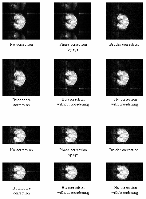
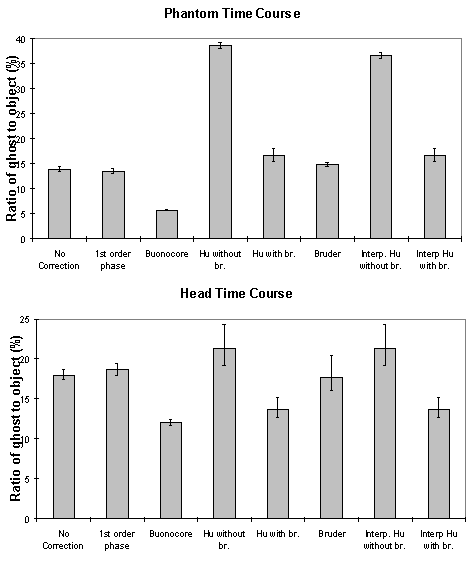
These methods were applied to a test fMRI data set of 64 volume images of a phantom and of a head, acquired over a time of 8 minutes. The first order phase correction method used was one where the signal intensity in the ghost region was minimised by applying the correction shown in equation 4.2. The Bruder correction and the two forms of the Hu correction were applied, such that one correction map was calculated, based on the first image in the set, and the same map applied to all images. Reference scans were also acquired at the end of the experiment in order to produce a correction map for every image, that was a linear interpolation between that for the first and that for the last. The graphs shown in Figure 4.10 show how well each technique corrected the ghost. The striking feature of these plots is that many of the methods, in particular the Hu correction without broadening, made the ghosting worse. This occurs in the columns in the image where the external r.f. interference is at its worse. The effect that this has on the image is shown in Figure 4.11a. Again the Buonocore method works the best in this situation for both head and ghost data. However, this technique does not always work, as is shown in Figure 4.11b. Since this correction is only based on those lines in which the ghost and image do not overlap, the method has failed where the signal intensity in the central rows is low. An appropriate choice of threshold can prevent low signal intensity having an adverse affect on image quality, but this highlights the care that must be used in applying any technique.
(a)  (b)
(b) 
Reducing the ghost artefact is not always easy. A technique that works well on one set of data fails completely on another, and because of this it is useful to be aware of all the possible corrections that could be applied. Since it does not require a reference scan, the Buonocore method would appear to be the most appropriate first choice, however more results obtained from using the method in practice will be necessary to confirm this.
As described in section 2.5.3, external r.f. radiation can cause bright dots of artefact to appear in the image. Provided that this interference is at a single discrete frequency, and the sampling is linear, only one or two pixels in the image will be affected and the image can be cleaned up by replacing these pixels by the average of their neighbours. Non-linear sampling however means that the single frequency interference is spread over a wide range of frequencies after Fourier transformation, and consequently appears as a line in the image. Not only does such interference spoil the appearance of the images, fluctuations in its intensity can cause problems with the analysis of the data. In order to cosmetically remove the interference in such a case, it is easier to re-grid the data, such that it appears that it was linearly sampled, and then to remove the few pixels which now contain the interference. The process is illustrated in Figure 4.12.
The most effective re-gridding of the time data occurs if each line in the image is expanded to fill a much larger grid, and then the gaps filled in by linear interpolation. The positions in the new grid of length n, of the existing N data points are found by summing under the sinusoidal gradient waveform, and finding the set of points X1...Xk...XN, such that
 .
.
(4.6)
The values of the intermediate points are obtained by linear interpolation, so that the intensity at the location X in the new grid is given by
 .
.
(4.7)
Re-gridding back from the linear to the sinusoidal grid simply involves extracting the values at the points X1...Xk...XN.
The exact pixels to remove are not easy to determine blindly. It is often the case that they are the brightest pixels, but not always, and because of this software was written so that the user could easily select the pixels that should be removed by looking at the re-gridded image. The application was written in the perl scripting language [9], with all the data manipulations and calculations carried out in C programs. The user selects the pixels to remove from the expanded image using the mouse.
Examples of data sets before and after cleaning up are shown in Figure 4.13.
(a) 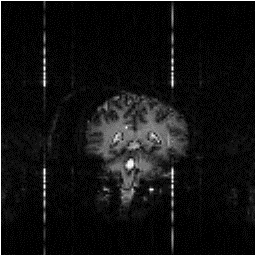 (b)
(b) 
The localisation of the activation response from an fMRI experiment depends on obtaining reference scans which highlight the anatomy of the subjects brain. For this purpose an inversion recovery image can be particularly beneficial, since the contrast in the grey and white matter regions of the brain can be altered by the use of a magnetisation inversion r.f. pulse and an appropriate delay before imaging (see section 2.4.1).
The pulse sequence diagram for a standard inversion recovery experiment is shown in Figure 4.14. At 3.0 Tesla the values of the inversion time, TI, required are 400 ms and 1200 ms for white matter null, and grey matter null respectively.
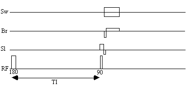
Acquiring the reference set, with a suitable number of repeats to gain sufficient signal to noise, can take several minutes. Much of this time is taken up by the inversion time delay. The fast inversion recovery sequence uses this time to invert other slices, before going back to image them, as shown in Figure 4.15.
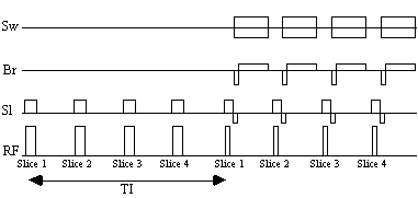
A constant repetition rate is chosen which is an integer multiple of the required inversion time. For example, to obtain grey matter null images with an inversion time of 1200 ms, four slices are inverted at a repetition rate of 300 ms. A comparison of images obtained using the conventional IR sequence with those obtained using the fast IR sequence shows no difference between the two, however for a typical set of white and grey matter images the fast sequence takes just over 5 minutes compared to 12 minutes for the standard IR method. The main limit to the speed of the fast IR acquisition is the rate of inversion pulses that it is safe to use, because of SAR considerations.
This reduction in time that the subject stays in the scanner helps to keep the subject motivated, and minimises discomfort, which in turn will reduce motion artefact.
If the results from fMRI experiments are to be reliable, comparable and efficiently obtained, it is necessary to standardise the way that such experiments are carried out. To this end, a standard fMRI protocol was written. The aim of this was to provide an experimental outline that contained the basic procedures that should be carried out, but could be adapted to fit the study in question. The standard fMRI protocol is given in Appendix A.
Correct configuration of the scanner is given purely as a reference, as it is assumed that the operator will be familiar with the operation of the 3.0 Tesla scanner [10]. The standard cylindrical phantom used on the 3.0 T scanner contains structure that can enable its orientation to be determined from the images. A standard orientation of the phantom is given to avoid confusion when looking at the images at a later date, and for this reason a phantom reference set of images is always stored with the data from that particular experiment. The stability of the scanner is tested each day that fMRI is carried out, by imaging a single slice of a phantom for about 5 minutes. A repetition rate of 10 seconds ensures that the effect of stimulated echoes does not interfere with the result. The stability can be calculated on a pixel by pixel basis by dividing the standard deviation of the pixel time course by its mean. The stability is regarded as satisfactory if this ratio is less than 0.5% throughout the phantom.
Anatomical reference scans are acquired with each data set, so that the precise location of the activation can be determined. If thick slices (> 1 cm) of the brain are to be imaged in the fMRI experiment, then it is better to acquire thinner slices for the reference scans, since the reduction in through slice susceptibility dephasing that this brings will improve the image quality considerably. A method for acquiring these thin slices such that they directly correspond to the thick slices is described in the protocol.
No details of how the stimulus paradigm should be designed are included in the standard protocol. This is because each paradigm may need to be developed depending on many factors such as the size of signal change observed on activation, how the stimulus is presented, how the subject is to respond, and the length of time a subject is able to stay in the scanner. For an initial experiment, a 16 cycle paradigm, with each cycle consisting of 16 seconds of rest and 16 seconds of activity has been shown to be reliable in a number of situations. The results presented later in this thesis, however, show that functional imaging of a single cognitive event is possible, and paradigms that exploit this may yield extra results over those obtained in an epoch based paradigm.
[1] Van Gelderen, P., Duyn, J. H., Liu, G. and Moonen, C. T. W. (1994) Optimal T2* weighting for BOLD-type Functional MRI of the Human Brain. Proc. Indian Acad. Sci. (Chem. Sci.) 106,1617-1624.
[2] Singh, M., Patel, P. and Khosla, D. (1996) Estimation of T2* in Functional Spectroscopy during Visual Stimulation. IEEE Trans. Nucl. Sci. 43,2037-2043.
[3] Menon, R. S., Ogawa, S., Tank, D. W. and Ugurbil, K. (1993) 4 Tesla Gradient Recalled Echo Characteristics of Photic Stimulation-Induced Signal Changes in the Human Primary Visual Cortex. Magn. Reson. Med. 30,380-386.
[4] Born, P., Rostrup, E. and Larsson, H. B. W. (1997) Dynamic R2* Mapping in Functional MRI. in Book of Abstracts, 5th Annual Meeting, International Society of Magnetic Resonance in Medicine p.1633.
[5] Bruder H., Fischer, H., Reinfelder, H.-E. and Schmitt, F. (1992) Image Reconstruction for Echo Planar Imaging with Nonequidistant k-Space Sampling. Magn. Reson. Med. 23,311-323.
[6] Hu, X., and Le, T. H. (1996) Artefact Reduction in EPI with Phase-encoded Reference Scan Magn. Reson. Med. 36,166-171.
[7] Mansfield, P. (1977) Multi-Planar Image Formation Using NMR Spin Echoes. J. Phys. C. 10,L55-L58.
[8] Buonocore, M. H. and Gao, L. (1997) Ghost Artefact Reduction for Echo Planar Imaging Using Image Phase Correction. Magn. Reson. Med. 38,89-100.
[9] See Wall, L. and Schwartz, R. Programming Perl, OReilly & Associates.
[10] Mansfield, P., Coxon, R. and Glover, P. (1994) Echo-Planar Imaging of the Brain at 3.0 T: First Normal Volunteer Results. J. Comput. Assist. Tomogr. 18,339-343.