The idea of localisation of function within the brain has only been accepted for the last century and a half. In the early 19th century Gall and Spurzheim, were ostracised by the scientific community for their so-called science of phrenology[1]. They suggested that there were twenty-seven separate organs in the brain, governing various moral, sexual and intellectual traits. The importance of each to the individual was determined by feeling the bumps on their skull. The science behind this may have been flawed, but it first introduced the idea of functional localisation within the brain which was developed from the mid 1800's onwards by clinicians such as Jackson [2] and Broca[3]. Most of the information available on the human brain came from subjects who had sustained major head wounds, or who suffered from various mental disorders[4]. By determining the extent of brain damage, and the nature of the loss of function, it was possible to infer which regions of the brain were responsible for which function.
Patients with severe neurological disorders were sometimes treated by removing regions of their brain. For example, an effective treatment for a severe form of epilepsy involved severing the corpus callosum, the bundle of nerve fibres which connect left and right cerebral hemispheres. Following the surgery patients were tested, using stimuli presented only to the left hemisphere or to the right hemisphere[5]. If the object was in the right visual field, therefore stimulating the left hemisphere, then the subject was able to say what they saw. However if the object was in the left visual field, stimulating the right hemisphere, then the subject could not say what they saw but they could select an appropriate object to associate with that image. This suggested that only the left hemisphere was capable of speech.
With the development of the imaging techniques of computerised tomography (CT) and magnetic resonance imaging it was possible to be more specific as to the location of damage in brain injured patients. The measurement of the electrical signals on the scalp, arising from the synchronous firing of the neurons in response to a stimulus, known as electroencephalography (EEG), opened up new possibilities in studying brain function in normal subjects. However it was the advent of the functional imaging modalities of positron emission tomography (PET), single photon emission computed tomography (SPECT), functional magnetic resonance imaging (fMRI), and magnetoencephalography (MEG) that led to a new era in the study of brain function.
In this chapter the mechanisms of the techniques mentioned above are outlined, together with an assessment of their strengths and weaknesses. Then an introduction to the physical and structural anatomy of the brain is given, and some of the terminology used in neurology is introduced. This is followed by a more detailed explanation of functional MRI and how such experiments are performed.
The imaging modalities of single photon emission computed tomography (SPECT) and positron emission tomography (PET) both involve the use of radioactive nuclides either from natural or synthetic sources. Their strength is in the fact that, since the radioactivity is introduced, they can be used in tracer studies where a radiopharmaceutical is selectively absorbed in a region of the brain.
The main aim of SPECT as used in brain imaging, is to measure the regional cerebral blood flow (rCBF). The earliest experiments to measure cerebral blood flow were performed in 1948 by Kety and Schmidt[6]. They used nitrous oxide as an indicator in the blood, measuring the differences between the arterial input and venous outflow, from which the cellular uptake could be determined. This could only be used to measure the global cerebral blood flow, and so in 1963 Glass and Harper[7], building on the work of Ingvar and Lassen[8], used the radioisotope Xe-133, which emits gamma rays, to measure the regional cerebral blood flow. The development of computed tomography in the 1970's allowed mapping of the distribution of the radioisotopes in the brain, and led to the technique now called SPECT[9].
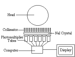
The radiotracer (or radiopharmaceutical) used in SPECT emits gamma rays, as opposed to the positron emitters used in PET. There are a range of radiotracers that can be used, depending on what is to be measured. For example I-123-3-quinuclidinyl 4-isodobenzilate is a neurotransmitter agonist which can be used for imaging receptors. For rCBF measurements Xe-133 can be introduced into the blood stream by inhalation. Detection is carried out using a gamma camera - a scintillation detector consisting of a collimator, a NaI crystal, and a set of photomultiplier tubes as shown in Figure 3.1.
By rotating the gamma camera around the head, a three dimensional image of the distribution of the radiotracer can be obtained by employing filtered back projection (as described in section 2.3.4). The radioisotopes used in SPECT have relatively long half lives (a few hours to a few days) making them easy to produce and relatively cheap. This represents the major advantage of SPECT as a brain imaging technique, since it is significantly cheaper than either PET or fMRI. However it lacks good spatial or temporal resolution, and there are safety aspects concerning the administration of radioisotopes to the subject, especially for serial studies.
Positron emission tomography[10] has two major advantages over SPECT, namely better spatial resolution and greater sensitivity. This comes from using positron emitters such as O-15 and F-18 as the radionuclide. When such nuclei decay they emit a positron, that is a particle with the same rest mass as an electron but with charge +1. Once the positron is emitted it travels a short distance before colliding with an electron. The annihilation of the two particles creates two photons each with energy 511 keV. In order to conserve momentum, the two photons are emitted at virtually 180 degrees to each other, and it is these photons that are detected in a ring of scintillators and photomultiplier tubes surrounding the head (Figure 3.2).
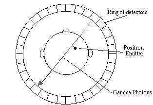
Opposite pairs of detectors are linked so as to register only coincident photons, thus defining a set of coincidence lines. Reconstruction of these lines by filtered back projection gives an image of the source of the annihilation. Since the detectors only record the site of the annihilation, resolution in a PET scanner is limited by the distance travelled by the positron through the tissue before it meets an electron. This fundamentally restricts the resolution of the scanner to 2 - 3 mm at best.
The positron emitters used in PET have short half lives, of the order of 2 - 100 minutes. This means that the isotopes must usually be made at the site of the scanner, using an expensive cyclotron. However, this short half life means that dynamic studies of brain function can be carried out using the technique.
Functional imaging studies using PET first appeared in 1984 with a study using C15O 2. Usually two cognitive states are imaged, one active and one resting, and by subtracting these two states a map of the regions of the brain responsible for that task made. PET is widely used as a tool for cognitive function, and much of the literature on brain function published in the last 10 years has used the technique. Positron emitting neurotransmitters such as F-18 labelled DOPA, mean that dopamine function can be followed in patients with Parkinson's disease. The main drawback of PET is it's use of radioisotopes, and its very high cost, however it's neurotransmitter mapping ability means that it will retain a role in the face of the less invasive, and more available fMRI.
Measuring the electrical signals from the brain has been carried out for several decades [11], but it is only more recently that attempts have been made to map electrical and magnetic activity. The electroencephalogram (EEG) is recorded using electrodes, usually silver coated with silver chloride, attached to the scalp and kept in good electrical contact using conductive electrode jelly. One or more active sites may be monitored relative to a reference electrode placed on an area of low response activity such as the earlobe. The signals are of the order of 50 microvolts, and so care must be taken to reduce interference from external sources, eye movement and muscle activity. Several characteristic frequencies are detected in the human EEG. For example, when the subject is relaxed the EEG consists mainly of frequencies in the range 8 to 13 Hz, called alpha waves, but when the subject is more alert the frequencies detected in the signal rise above 13Hz, called beta waves. Measurements of the EEG during sleep have revealed periods of high frequency waves, known as rapid eye movement (REM) sleep which has been associated with dreaming.
The EEG can also be measured in response to some regularly repeated stimulus such as the pattern reversal of a projected checkerboard, or more complicated task such as number memorising and recall. The signal, from each electrode, in response to the stimulus is recorded and averaged together over a number of trials. The response is characterised by the delay, or latency, of the peak of the signal from the presentation of the stimulus. This is of the order of milliseconds for brain stem responses and 100's of milliseconds for cortical responses. For example a commonly detected response to an oddball stimulus, the P300, has a latency of 300 ms. Having found an electrical signal of interest, the magnitude of the peak can be mapped across the scalp giving an idea of the source. The major limitation of studying brain function using EEG is that the signals measured are recorded on the scalp, which may not represent the activity in the underlying cortex. However since the technique is very cheap and safe, it has many uses and can be involved in studies where the scanning techniques could not, such as continuous monitoring during sleep.
Since the magnetic signals from the firing of the neurons do not need to be conducted to the scalp, measuring them gives much greater signal localisation than measuring the currents themselves. This is the basis of the much newer technique of magnetoencephalography (MEG). The first successful measurements of these magnetic fields were made by Cohen in 1972 [12]. The magnitude of the magnetic signals, resulting from the electrical firing of the neurons is of the order of 10-13 Tesla, for 1 million synchronously active synapses. Such small signals are picked up using a superconducting quantum interference device (SQUID) magnetometer (Figure 3.3).
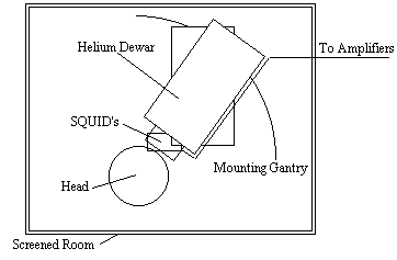
Interference from external sources is a major problem with MEG, and the magnetometer must be sited in a magnetically shielded room. Current magnetometers have as many as 120 SQUIDS covering the scalp.
MEG experiments are carried out in much the same way as their EEG counterpart. Having identified the peak of interest, the signals from all the detectors are analysed to obtain a field map. From this map an attempt can be made to ascertain the source of the signal by solving the inverse problem. Since the inverse problem has no unique solution, assumptions need to be made, but providing there are only a few activated sites, close to the scalp then relatively accurate localisation is possible, giving a resolution of the order of a few millimetres.
MEG has the advantage over EEG that signal localisation is, to an extent, possible, and over PET and fMRI in that it has excellent temporal resolution of neuronal events. However MEG is costly and its ability to accurately detect events in deeper brain structures is limited.
Since functional magnetic resonance imaging (fMRI) is the subject of this thesis, little will be said in this section as to the mechanisms and applications of the technique, as this is covered later in the chapter. The purpose of this section is to compare fMRI to the other modalities already mentioned, and also to consider the related, but distinct technique of magnetic resonance spectroscopy (MRS).
During an fMRI experiment, the brain of the subject is scanned repeatedly, usually using the fast imaging technique of echo planar imaging (EPI). The subject is required to carry out some task consisting of periods of activity and periods of rest. During the activity, the MR signal from the region of the brain involved in the task normally increases due to the flow of oxygenated blood into that region. Signal processing is then used to reveal these regions. The main advantage of MRI over its closest counterpart, PET, is that it requires no contrast agent to be administered, and so is considerably safer. In addition, high quality anatomical images can be obtained in the same session as the functional studies, giving greater confidence as to the source of the activation. However, the function that is mapped is based on blood flow, and it is not yet possible to directly map neuroreceptors as PET can. The technique is relatively expensive, although comparable with PET, however since many hospitals now have an MRI scanner the availability of the technique is more widespread.
FMRI is limited to activation studies, which it performs with good spatial resolution. If the resolution is reduced somewhat then it is also possible to carry out spectroscopy, which is chemically specific, and can follow many metabolic processes. Since fMRS can give the rate of glucose utilisation, it provides useful additional information to the blood flow and oxygenation measurements from fMRI, in the study of brain metabolism.
The brain imaging techniques that have been presented in this chapter all measure slightly different properties of the brain as it carries out cognitive tasks. Because of this the techniques should be seen as complementary rather than competitive. All of them have the potential to reveal much about the function of the brain and they will no doubt develop in clinical usefulness as more about the underlying mechanisms of each are understood, and the hardware becomes more available. A summary of the strengths and weaknesses of the techniques is presented in Table 3.1.
| Technique | Resolution | Advantages | Disadvantages |
| SPECT | 10 mm | Low cost Available |
Invasive Limited resolution |
| PET | 5 mm | Sensitive Good resolution Metabolic studies Receptor mapping |
Invasive Very expensive |
| EEG | poor | Very low cost Sleep and operation monitoring |
Not an imaging technique |
| MEG | 5 mm | High temporal resolution | Very Expensive Limited resolution for deep structures |
| fMRI | 3 mm | Excellent resolution Non-invasive |
Expensive Limited to activation studies |
| MRS | low | Non-invasive metabolic studies |
Expensive Low resolution |
Since much of this thesis makes references to brain anatomy and function, this section deals with the terminology used in the discipline of neurology. There are four sections covering brain anatomy, brain cellular structure and brain function. Further reference can be obtained from the many good books on brain biochemistry and neuroanatomy [13,14,15].
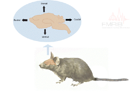
In order to describe the position of structures relative to each other in the brain, neurology has a number of terms of direction, many of which are derived from the Latin or Greek. There are two axes which describe the organisation of the central nervous system (CNS). These are most easily understood in animals with the spinal cord running horizontally rather than vertically. In this case the rostral-caudal axis runs from nose to tail, and the dorsal-ventral axis runs perpendicularly to this as shown in Figure 3.4a. Now using this system in the human spinal cord, 'top to bottom' is 'caudal to rostral', and 'back to front' is 'dorsal to ventral' (Figure 3.4b). In the human brain however these axes turn through 90 degrees, so the front of the brain is rostral, top is dorsal, and base is ventral.
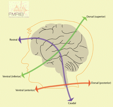
In addition to these labels, there is another perpendicular set of axes which is the same for spinal cord and brain, that is anterior=front, posterior=back, superior=top, inferior=bottom.
The midline runs down the centre of the brain, separating left from right. If two structures are on the same side of the midline, they are said to be ipsilateral, whereas they are contralateral if they are on opposite sides. When comparing two structures, the one closest to the midline is medial, as opposed to the other which is lateral.
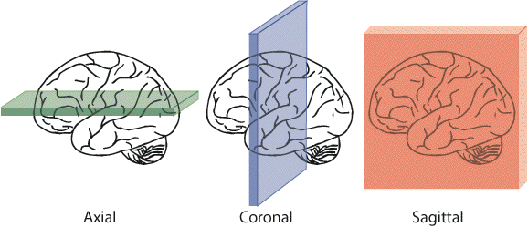
When viewing sections through the brain, three mutually perpendicular planes are commonly considered, as shown in Figure 3.5. These are axial (or transverse) coronal, and sagittal.
The neuron is the basic functional unit of the nervous system. The brain consists of several hundred billion neurons, communicating by billions of interconnections. All neurons consist of four distinct parts: cell body, dendrites, axons and axon terminals (Figure 3.6).
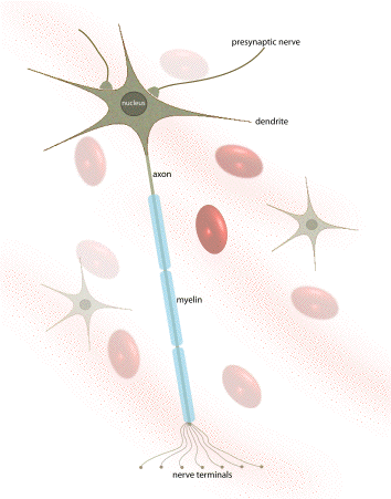
The cell body (or soma) contains the nucleus of the cell, as well as the essential cellular organelles, such as the energy generating mitochondria. The cell body has many branches, called dendrites, which receive signals from other cells, and are often covered in dendritic spines. Extending from the cell body in one direction is an axon. The length of axons can be several centimetres or longer. Axons carry information from one neuron to another, and are terminated at the synaptic knob, which is attached to the dendrites or cell body of another neuron. Signals are transferred across the synapse by means of a chemical neurotransmitter.
Signals travel along the axon by generating and propagating an action potential. This is produced by letting the delicate balance of sodium, potassium and chloride ions across the cell membrane be altered, thus generating an electrical signal that flows along the axon. If the axon is coated in a fatty sheath, called myelin, the signal travels at higher speeds of anything up to 120 ms-1. When the signal reaches the synapse, the synaptic knob emits a neurotransmitter which acts either to encourage the next neuron to 'fire' (excitatory) or discourage the neuron to fire (inhibitory).
The CNS contains a number of different types of neurons, which are tailored to the job they perform. Signals from sensory receptors over the body feed along the spinal cord to the brain, and signals are sent from the brain to make muscles contract. Many medical conditions are caused by the failure of the CNS to function correctly, for example in Parkinson's disease there is a deficiency of the neurotransmitter dopamine.
For every neuron in the CNS there are also ten glial cells. These cells provide support for neurons, for example the microglia which perform a scavenger role, and oligodendrocytes which form the myelin sheath around the axons.
The central nervous system consists of the spinal cord and the brain. The brain is then further divided into the forebrain, midbrain, and hindbrain (Figure 3.7).
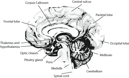
The largest region is the forebrain, which contains the cerebral hemispheres, the corpus callosum, thalamus, hypothalamus, and hippocampus. the hindbrain consists of the cerebellum, pons, and medulla. The structure of each of these is described below.
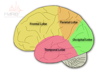
The cerebrum is divided into two hemispheres, the left and the right, separated by the longitudinal fissure. Anatomically these are identical in form, each being split into four lobes; the frontal lobe, the parietal lobe on the top, the temporal lobe on the side, and the occipital lobe at the back (Figure 3.8). The frontal and parietal lobes are separated by the central sulcus, and the temporal lobe separated by the lateral fissure. The corpus callosum joins left and right hemispheres.
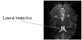
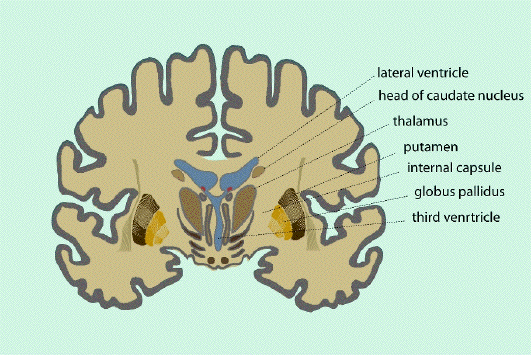
Under the surface of the cerebral hemispheres are bundles of fibres, the basal ganglia, connecting together many regions of the cerebral cortex. The thalamus, hypothalamus and hippocampus are located at the centre of the forebrain, just above the midbrain (Figure 3.10). At the rear of the brain is a more tightly folded structure called the cerebellum, which is connected to the pons, the medulla, and finally the spinal cord.
The functional organisation of much of the brain is poorly understood. However many of the regions involved in sensory and motor function have been identified.
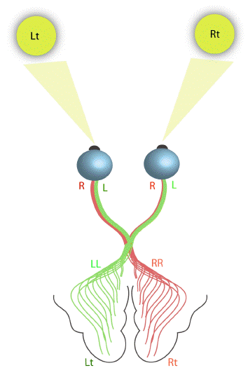
The primary visual cortex is located in the occipital lobe, which deals with the reception and interpretation of vision. The right visual field is mapped on to the left cerebral hemisphere, and the left visual field on to the right hemisphere (Figure 3.11). The signals from the retina travel along the optic tracts, which cross over at the optic chiasm.

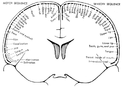
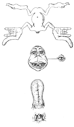
The organisation of the somatosensory cortex shows similarity to a map of the surface of the body[16]. This is illustrated in what is known as the sensory homunculus (Figure 3.13). A much greater part of the somatosensory cortex is associated with the hand and face, compared to regions not so important in tactile tasks such as the leg. Similarly there is a motor homunclus which illustrates the layout of the motor cortex. The hand is given much more cortical surface in the motor cortex than in the somatosensory cortex, representing the highly sophisticated tasks that the hands perform.
All the regions mentioned so far are primary cortices because they are most closely involved with the brain's input and output. Much of the rest of the brain is given over to integrating these stimuli, and interpreting how to respond. The regions responsible for these more abstract tasks are termed secondary (Figure 3.14). For example, the secondary motor regions, which are more anterior in the frontal lobes to the primary motor cortex, are responsible for planning and initiating motion, and the secondary visual area, close to the primary visual cortex is involved in interpreting colours and movement in the visual information. The tertiary areas, or association cortices, are responsible for the higher brain functions such as interpretation and memory.

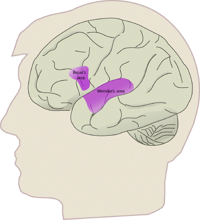
Some specific regions of interest are those responsible for speech, which are located in the left hemisphere of most people. Broca's area is in the lower part of the frontal lobe (Figure 3.15), and is involved in the formation of sentences, and Wernicke's area, located in the temporal lobe is involved in the comprehension of speech.
This is just a brief sketch of brain function as it is understood at present. New literature is appearing at a rapid pace, confirming and evolving the models. The motor system is covered in more detail in Chapter 7.
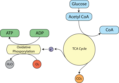
The biochemical reactions that transmit neural information via action potentials and neurotransmitters, all require energy. This energy is provided in the form of ATP, which in turn is produced from glucose by oxidative phosphorylation and the Kreb's cycle (Figure 3.16).
As ATP is hydrolysed to ADP, energy is given up, which can be used to drive biochemical reactions that require free energy. The production of ATP from ADP by oxidative phosphorylation is governed by demand, so that the energy reserves are kept constant. That is to say, the rate of this reaction depends mainly on the level of ADP present. This means that the rate of oxygen consumption by oxidative phosphorylation is a good measure of the rate of use of energy in that area.
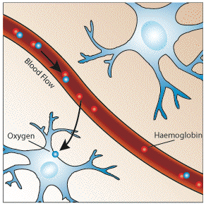
The oxygen required by metabolism is supplied in the blood. Since oxygen is not very soluble in water, the blood contains a protein that oxygen can bind to, called haemoglobin. The important part of the haemoglobin molecule is an iron atom, bound in an organic structure, and it is this iron atom which gives blood it's colour. When an oxygen molecule binds to haemoglobin, it is said to be oxyhaemoglobin, and when no oxygen is bound it is called deoxyhaemoglobin.
To keep up with the high energy demand of the brain, oxygen delivery and blood flow to this organ is quite large. Although the brain's weight is only 2% of the body's, its oxygen consumption rate is 20% of the body's, and blood flow 15%. The blood flow to the grey matter, which is a synapse rich area, is about 10 times that to the white matter per unit volume. Regulation of the regional blood flow is poorly understood, but it is known that localised neural activity results in a rapid selective increase in blood flow to that area.
Since regional blood flow is closely related to neural activity, measurement of the rCBF is useful in studying brain function. It is possible to measure blood perfusion with MRI, using techniques similar to those mentioned in section 2.4.4. However there is another, more sensitive, contrast mechanism which depends on the blood oxygenation level, known as blood oxygen level dependent (BOLD) contrast. The mechanisms behind the BOLD contrast are still to be determined, however there are hypotheses to explain the observed signal changes.
Deoxyhaemoglobin is a paramagnetic molecule whereas oxyhaemoglobin is diamagnetic. The presence of deoxyhaemoglobin in a blood vessel causes a susceptibility difference between the vessel and its surrounding tissue. Such susceptibility differences cause dephasing of the MR proton signal [18], leading to a reduction in the value of T2*. In a T2* weighted imaging experiment, the presence of deoxyhaemoglobin in the blood vessels causes a darkening of the image in those voxels containing vessels[19,20]. Since oxyhaemoglobin is diamagnetic and does not produce the same dephasing, changes in oxygenation of the blood can be observed as the signal changes in T2* weighted images [21,22,23].
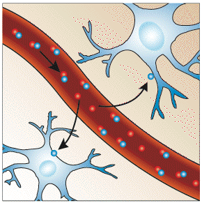
It would be expected that upon neural activity, since oxygen consumption is increased, that the level of deoxyhaemoglobin in the blood would also increase, and the MR signal would decrease. However what is observed is an increase in signal, implying a decrease in deoxyhaemoglobin. This is because upon neural activity, as well as the slight increase in oxygen extraction from the blood, there is a much larger increase in cerebral blood flow, bringing with it more oxyhaemoglobin (Figure 3.17). Thus the bulk effect upon neural activity is a regional decrease in paramagnetic deoxyhaemoglobin, and an increase in signal.
 |
 |
| Resting | Activated |
The study of these mechanisms are helped by results from PET and near-infrared spectroscopy (NIRS) studies. PET has shown that changes in cerebral blood flow and cerebral blood volume upon activation, are not accompanied by any significant increase in tissue oxygen consumption[24]. NIRS can measure the changes in concentrations of oxy- and deoxyhaemoglobin, by looking at the absorbency at different frequencies. Such studies have shown an increase in oxyhaemoglobin, and a decrease deoxyhaemoglobin upon activation. An increase in the total amount of haemoglobin is also observed, reflecting the increase in blood volume upon activation [25].
The time course for the BOLD signal changes is delayed from the onset of the neural activity by a few seconds, and is smooth, representing the changes in blood flow that the technique detects. This is termed the 'haemodynamic response' to the stimulus. There have also been observations of an initial small 'dip' in signal before and after the larger increase in signal [26,27], possibly reflecting a transient imbalance between the metabolic activity and blood flow.
The discovery of the BOLD effect led to many groups trying to map brain activation using the technique. The first MR human brain activation study used an introduced contrast agent to map the visual cortex[28]. Soon after that the BOLD effect was used to map visual and motor function [29,30]. References to the many early fMRI experiments can be found in the review articles on the subject [31,32].
To study brain function using fMRI it is necessary to repeatedly image the brain, whilst the subject is presented with a stimulus or required to carry out some task. The success of the experiment is dependent on three aspects; the scanning sequence used, the design of the stimulus paradigm, and the way the data is analysed.
The magnitude of the static field used is critical to the percentage signal change obtained on activation. This is because susceptibility differences have a greater signal dephasing effect at higher fields. The earliest fMRI studies were carried out at 1.5 Tesla, but now the forefront research facilities use 3 to 4 Tesla scanners. As field strength increases the magnitude of the BOLD contrast increases more rapidly than system noise, so it would appear that higher field strengths are desirable [33], however the image quality will be reduced at higher field.
The most important aspect of the imaging sequence is that it must produce T2* weighted images. This means that a gradient echo is most commonly used, however spin echo sequences still show BOLD contrast because of diffusion effects. Most research is carried out using EPI since its fast acquisition rate allows the activation response to short stimuli to be detected. EPI also has the benefit of reduced artefact from subject motion.
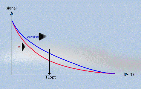
The amount of T2* weighting in the image is dependent on the echo time TE. If TE is too short, there will be little difference in the T2* curves for the activated state and the resting state, however if TE is too long then there will be no signal from either state. To obtain the maximum signal change for a region with a particular value of T2*, the optimal value of echo time can be shown to be equal to the T2* value of that tissue (Figure 3.18).
The contrast to noise ratio of the BOLD signal also depends on voxel size and slice thickness. Smaller voxels have less proton signal due to the reduced number of spins, however larger voxels may reduce the contrast to noise ratio by partial volume effects. This occurs if the signal changes on activation come from only a small region within the voxel, and so makes less of an impact on the total signal change in that voxel.
During the scanning there are a number of physiological effects that can affect results. These include cardiac pulsation, respiration and general subject movement. All these problems can be dealt with in two ways, either at the time of scanning or in image post processing. Cardiac or respiratory gating, that is triggering the scanner at one part of the cardiac cycle can be used, although this introduces artefact due to changes in the spin saturation. Postprocessing strategies have been proposed and are probably the best way to deal with this problem [34]. Subject movement can also reduce contrast to noise in fMRI images, and introduce artefact in the activation maps if the movement is stimulus correlated. This problem is often solved both by restraining the head of the subject and by using a postprocessing registration algorithm.
Another source of artefact in fMRI is the signal coming from draining veins. Since gradient echo images are sensitive to vessels of diameters from micrometers to millimetres, it can be difficult to distinguish between signals from the tissue and that from the veins, which could be some distance away from the activation site [35]. There is also the problem that blood flowing into the imaging slice may be stimulus correlated. One way to reduce the signal from large vessels would be to use a spin echo sequence. This is sensitive to T2 effects only and eliminates the dephasing effects from the large vessels [36,37]. Using a spin echo sequence will result in some reduction in genuine tissue BOLD signal, so often it is better to acquire a separate set of images which are sensitive to large vessels, and use this to decide whether to reject the signal.
The choice of the optimum parameters for fMRI is always a compromise, and often depends more on what is available than what is desirable. More is said on the optimisation of MRI for brain imaging in Chapter 4.
As important as choosing the imaging parameters for a good experiment is designing the stimulus paradigm. A lot of experience has come from EEG and PET, but since fMRI has a temporal resolution somewhere between these two techniques new approaches can be taken. There are many issues in paradigm design, so only an overview will be given here, with more specific examples of the adaptation of paradigms given in Chapter 7.
The earliest fMRI experiments were much in the form of PET studies, that is to say a set of resting images were acquired and then a set of activation images, and one set subtracted from the other. However since the BOLD contrast is relatively rapid in its onset and decay (of the order of a few seconds) it is possible to follow time courses for much shorter events occurring more frequently.
The most common stimulus presentation pattern is that of regular epochs of stimulus and rest, usually labelled 'on' and 'off'. The duration of these epochs needs to be long enough to accommodate the haemodynamic response, and so a value of at least 8 seconds, or more commonly 16 seconds is chosen. These epochs are repeated for as long as is necessary to gain enough contrast to noise to detect the activation response. The total experimental duration however must be a balance between how long the subject can comfortably lie still without moving, and the number of data points required to obtain enough contrast to noise. There are often some technical limitations to the experimental duration, and there is the possibility of the subject habituating to the stimulus causing the BOLD contrast to reduce with time.
Instead of epochs of stimuli, it is possible to use single events as a stimulus, much in the same way that EEG or MEG does. Again due to the haemodynamic response, these must be separated by a much longer period of time than would be required for EEG, but since this type of stimulus presentation has the major advantage of being able to separate out the relative timings of activations in different areas of the brain. One of the major disadvantages of single event paradigms is that the experiments need to be much longer than their epoch based counterparts, in order to gain the necessary contrast to noise. More is said on the design of single event paradigms in Chapter 7.
The choice of stimulus is very critical. For example, to activate the primary visual cortex is straightforward, but to determine the regions responsible for colour discrimination is more difficult. Ideally it is necessary to design the 'on' and 'off' epoch such that there is only one well defined difference between them, which will only activate those brain regions responsible for the single task. This is not always possible and so a hierarchy of experiments often need to be performed. For example to identify the regions responsible for task A, an experiment can be performed which involves task A and task B, and then one which only involves task B. The regions responsible for task A would presumably be those activated in the first experiment but not the second. This assumes that the system is a linear one, which may not be the case, or there could be some unaccounted for differences in the two paradigms, which could affect the result.
Another problem particularly when dealing with cognitive events such as memory, is that some stimulus must be presented, usually visually, and a subject response given, usually involving motor action. These must either be compensated for by being included in the 'off' period as well, or another experiment must be performed later which involves similar stimulus and response, but not the cognitive task performed in the original experiment. Alternatively the stimulus may be presented in a different way, aurally for example, and response given orally, and those regions common to both stimulus presentation types can be assumed to be responsible for the cognitive task of interest.
There are a few stimuli which are hard to present in an fMRI experiment. One obvious one is an auditory stimulus. The rapid imaging scanners are very noisy in their operation, especially if EPI is used. Although aural cues can usually be heard, they are not as easily detected as visually presented cues, and detecting activations in the primary auditory cortex is very difficult since there is always a large amount of ambient sound throughout both 'on' and 'off' periods. Requiring the subject to respond orally is also problematic since this almost always results in head movement, which would be concurrent with the stimulus. All response movements required need to be small to reduce head motion during the scanning.
The subject needs to have good instructions, and be reminded to lie still, and to concentrate. Many stimuli give better activation if a response is required to be made. There is much more that could be said on good paradigm design, and much is still being learnt, however care must always be taken and much thought be given for any new experiment.
The statistical analysis of fMRI data is the subject of the sixth chapter of this thesis, and covered in much more detail there. However to complete this section on functional MRI a few of the common analysis strategies are given here.
The analysis of fMRI data falls into two parts. Firstly the raw data must be analysed to produce an image showing the regions of activation and secondly, some level of significance must be calculated so that the probability of any of producing such a result purely by chance is suitably low [38].
The most straightforward way to analyse the data is to subtract the mean 'off' image from the mean 'on' image. This has the disadvantage that any small movement of the head can drastically change the pixel intensity at the boundaries of the image. This can give rise to a ring of apparent activation near the brain boundaries. To reduce this effect, and to give a statistic of known distribution, a student's t-test can be used. This biases the result against pixels in either 'on' or 'off' set with very large variability, and so can reduce movement artefact. An image where each pixel is assigned a value based on the output of a statistical test is commonly called a statistical parametric map.
Another commonly used technique is that of correlation coefficient mapping. Here the time response of the activation to the stimulus is predicted, usually with some knowledge of the haemodynamic response, and the correlation coefficient between each pixel time course and this reference function is calculated.
Other methods that have been used include Fourier transformation, which identifies pixels with a high Fourier component an the frequency of stimulus presentation, principal component analysis, which locates regions in the brain which show synchronous activity using eigenfunctions, clustering techniques, which again look for synchrony using iterative methods, and various non-parametric tests which do not require the assumption of normality in the signal distribution. All these have their various strengths and weaknesses, and no doubt new methods or variants will be developed in due course. The main criteria for any technique however is simplicity, speed, statistical validity, and sensitivity.
Having obtained a statistical map it is necessary to display the regions of activation, together with some estimate as to the reliability of the result. If the distribution of the statistic, under the null hypothesis of no activation present, is known, then statistical tables can be used to threshold the image, showing only those pixels which show strong stimulus correlation. When displaying the results as an image usually of several thousand pixels, it is necessary to account for multiple comparisons, since the probability of any one pixel in the image being falsely labelled as active is much greater than the probability of a lone pixel being falsely labelled. There are several ways to account for this, for example the Bonferoni correction or the theory of Gaussian random fields, and this topic is explored in more detail in Chapter 6.
[1] Gall, F. J. and Spurzheim, J. C. (1810) `Anatomie und Physiologie des Nervensystems im Allgemeinen und des Gehirns insbesondere', F. Schoell, Paris.
[2] Jackson, J. H. (1931) `Selected Writings of John Hughlings Jackson', Hodder and Stoughton, London.
[3] Broca, P. (1861) Sur le siège de la faculté du langage articulé. Bull. Soc. anat. de Paris, 2 Serie, 6,355.
[4] Penfield, W. and Rasmussen, T. (1952) `The Cerebral Cortex of Man'. Macmillan, New York.
[5] Sperry, R. W. (1968) Hemisphere Deconnection and Unity in Conscious Awareness. American Psychologist 23,723-733.
[6] Kety, S. S. and Schmidt, C. F. (1948) The Nitrous Oxide Method for the Quantitative Determination of Cerebral Blood Flow in Man: Theory, Procedure and Normal Values. J. Clin. Invest. 27,476-483.
[7] Glass, H. I. and Harper, A. M. (1963) Measurement of Regional Blood Flow in Cerebral Cortex of Man through Intact Skull. Br. Med. J. 1,593.
[8] Ingvar, D. H. and Lassen, N. A. (1961) Quantitative Determination of Regional Cerebral Blood-Flow. Lancet 2,806-807.
[9] Kuhl, D. E. and Edwards R. Q. (1963) Image Separation Radioisotope Scanning. Radiology 80,653-661.
[10] Fox, P. T., Mintun, M. A., Raichle, M. E. and Herscovitch, P. (1984) A Noninvasive Approach to Quantitative Functional Brain Mapping with H215O and Positron Emission Tomography. J. Cereb. Blood Flow Metab. 4,329-333.
[11] Berger, H. (1929) Über das elektrenkephalogramm des menschen. Arch. Psychiatr Nervenkr 87, 527-570.
[12] Cohen, D. (1972) Magnetoencephalography: Detection of the Brain's Electrical Activity with a Superconducting Magnetometer. Science 175,664-666.
[13] Bachelard, H. S. (1981) `Brain Biochemistry'. Chapman & Hall.
[14] Kandel, E. R., Schwartz, J. H. and Jessel, T. M. (1991) `Principles of Neural Science' Appleton & Lange.
[15] Martin, J. H. (1996) `Neuroanatomy', Appleton & Lange.
[16] Penfield, W. G. and Rasmussen T. (1952) `The Cerebral Cortex of Man', Macmillan, New York.
[17] Pauling, L. and Coryell, C. D. (1936) The Magnetic Properties and Structure of Hemoglobin, Oxyhemoglobin and Carbonmonoxyhemoglobin Proc. Natl. Acad. Sci. USA 22,210-216.
[18] Thulborn, K. R., Waterton, J. C., Matthews, P. M. and Radda, G. K. (1982) Oxygen Dependence of the Transverse Relaxation Time of Water Protons in Whole Blood at High Field. Biochim. Biophys. Acta. 714, 265-270.
[19] Ogawa, S., Lee, T. M., Nayak., A. S. and Glynn, P. (1990) Oxygenation-Sensitive Contrast in Magnetic Resonance Image of Rodent Brain at High Magnetic Fields. Magn. Reson. Med. 14, 68-78.
[20] Ogawa, S. and Lee, T. M. (1990) Magnetic Resonance Imaging of Blood Vessels at High Fields: In Vivo and in Vitro Measurements and Image Simulation. Magn. Reson. Med. 16, 9-18.
[21] Ogawa, S., Lee, T. M., Kay, A. R. and Tank, D. W. (1990) Brain Magnetic Resonance Imaging with Contrast dependent on Blood Oxygenation. Proc. Natl. Acad. Sci. USA 87, 9868-9872.
[22] Turner, R., Le Bihan, D., Moonen, C. T. W., Despres, D. and Frank, J. (1991) Echo-Planar Time Course MRI of Cat Brain Oxygenation Changes. Magn. Reson. Med. 22, 159-166.
[23] Jezzard, P., Heinemann, F., Taylor, J., DesPres, D., Wen, H., Balaban, R.S., and Turner, R. (1994) Comparison of EPI Gradient-Echo Contrast Changes in Cat Brain Caused by Respiratory Challenges with Direct Simultaneous Evaluation of Cerebral Oxygenation via a Cranial Window. NMR in Biomed. 7,35-44.
[24] Fox, P. T., Raichle, M. E., Mintun, M. A. and Dence, C. (1988) Nonoxidative Glucose Consumption During Physiologic Neural Activity. Science 241, 462-464.
[25] Villringer, A., Planck, J., Hock, C., Schleinkofer, L. and Dirnagl, U. (1993) Near Infrared Spectroscopy (NIRS): A New Tool to Study Hemodynamic Changes During Activation of Brain Function in Human Adults. Neurosci. Lett. 154, 101-104.
[26] Ogawa, S, Tank, D. W., Menon, R., Ellermann, J. M., Kim S. G., Merkle, H. and Ugurbil, K. (1992) Intrinsic Signal Changes Accompanying Sensory Stimulation: Functional Brain Mapping with Magnetic Resonance Imaging. Proc. Natl. Acad. Sci. USA 89, 5951-5955.
[27] Ernst, T. and Hennig, J. (1994) Observation of a Fast Response in Functional MR. Magn. Reson. Med. 32,146-149.
[28] Belliveau, J. W., Kennedy, D. N., McKinstry, R. C., Buchbinder, B. R., Weisskoff, R. M., Cohen, M. S., Vevea, J. M., Brady, T. J. and Rosen, B. R. (1991) Functional Mapping of the Human Visual Cortex by Magnetic Resonance Imaging. Science 254, 716-719.
[29] Kwong, K. K., Belliveau, J. W., Chesler, D. A., Goldberg, I. E., Weisskoff, R. M., Poncelet, B. P, Kennedy, D. N., Hoppel, B. E., Cohen, M. S., Turner, R., Cheng, H. M., Brady, T. J. and Rosen, B. R. (1992) Dynamic Magnetic Resonance Imaging of Human Brain Activity During Primary Sensory Stimulation. Proc. Natl. Acad. Sci. USA 89, 5675-5679.
[30] Bandettini, P. A., Wong, E. C., Hinks, R. S., Tikofsky, R. S. and Hyde, J. S. (1992) Time Course EPI of Human Brain Function During Task Activation. Magn. Reson. Med. 25,390-397.
[31] Kwong, K.K. (1995) Functional Magnetic Resonance Imaging with Echo Planar Imaging. Magnetic Resonance Quarterly 11,1-20.
[32] Cohen, M.S. and Bookheimer, S. Y. (1994) Localization of Brain Function using Magnetic Resonance Imaging. Trends in Neuroscience 17,268-277.
[33] Turner, R., Jezzard, P., Wen, H., Kwong, K. K., Le Bihan, D., Zeffiro, T. and Balaban, R. S. (1993) Functional Mapping of the Human Visual Cortex at 4 and 1.5 Tesla Using Deoxygenation Contrast EPI. Magn. Reson. Med. 29,277-279.
[34] Le, T. H and Hu, X. (1996) Retrospective Estimation and Correction of Physiological Artifacts in fMRI by Direct Extraction of Physiological Activity from MR Data. Magn. Reson. Med. 35,290-298.
[35] Gao, J. H., Miller, I., Lai, S., Xiong, J. and Fox, P. T. (1996) Quantitative Assessment of Blood Inflow Effects in Functional MRI Signals. Magn. Reson. Med. 36,314-319.
[36] Fisel, C. R., Ackerman, J. L., Buxton, R. B., Garrido, L., Belliveau, J. W., Rosen, B. R. and Brady, T. J. (1991) MR Contrast Due to Microscopically Heterogeneous Magnetic Susceptibility: Numerical Simulations and Applications to Cerebral Physiology. Magn. Reson. Med. 17,366-347.
[37] Hykin, J., Bowtell, R., Mansfield, P., Glover, P., Coxon, R., Worthington, B. and Blumhardt, L. (1994) Functional Brain Imaging using EPI at 3T. Magma 2,347-349.
[38] Bandettini, P. A., Jesmanowicz, A., Wong, E. C. and Hyde, J. S. (1993) Processing Strategies for Time-Course Data Sets in Functional MRI of the Human Brain. Magn. Reson. Med. 30,161-173.