Signal and Image Processing Practical
Overview
This practical requires Python. Go through the page and execute the listed commands in your IDE of choice (you can copy-paste). Don't click on the "answers" links until you have thought hard about the question. Raise your hand should you need any help.
Required modules:
This practical requires the following Python modules:
- numpy
- matplotlib
- scipy
- skimage
Contents:
- Fourier analysis
- Learn basics of FFT in 1D (signals) and 2D (images)
- Filtering
- Learn to implement linear filters using convolution
- Image reconstruction
- Fourier/Radon transforms and image reconstruction
Fourier analysis
To start with, let us create some simple 1D signals and examine their Fourier transforms. In this first example, we will check the frequency content of a simple periodic signal.
Generate a cosine signal with given magnitude, frequency, sampling rate, and duration:
import numpy as np
import matplotlib.pylab as plt

mag  = 2;     # magnitude (arbitrary units)
freq = 5;     # frequency in Hz
samp = 100;   # sampling rate in Hz

t = np.arange(0.0,1.0,1.0/samp)  # time (1s of data)
N = len(t)                       # store the number of time points

x = mag*np.cos(2*np.pi*freq*t)   # the signal equation
plt.plot(t,x,'.-')
plt.show()
If you run the code above, you can see a nice cosine function. Make sure you understand the distinction between the sampling rate (in this case number of data points per second) and the frequency of the signal (number of cycles per second). In this case, since we have generated a signal that has a duration of 1 second, you should be able to easily count the number of cycles per second :)
Now, let us immediately look at the Fourier transform of this signal.
y = np.fft.fft(x);               # do Fast Fourier Transform
f = np.linspace(0.0,N-1.0,N);    # vector of frequencies for plotting

plt.plot(f,np.abs(y),'.-');      # plotting the magnitude of the FFT
plt.show()
This plot is called a powerspectrum. The first peak coincides with the frequency of the cosine function (check this). The second peak is redundant (for mathematical reasons). Therefore, from now on we will only display the first half of the fourier transform:
plt.plot(f[:N//2],np.abs(y[:N//2]))   # plotting half of the fft results
plt.xlabel('Freq (Hz)')               # labelling x-axis
plt.show()
Notice how the peak of the powerspectrum corresponds exactly to the frequency of the original signal. Now what happens to the powerspectrum when we:
- Change the frequency of the signal? Answer
- Change the magnitude of the signal? Answer
- Change the phase of the signal? Answer
- Change the sampling rate? Answer
Now let's do the opposite to the above. Instead of creating a
signal and looking at its FFT, we are going to create an FFT and
look at its signal. We will use the inverse FFT function in Numpy
(ifft).
We will create two signals, one that is the magnitude and one that is the phase, and we will look at the inverse fourier transform of these:
mag    = np.zeros(100)
mag[3] = 1               # spike in the magnitude at freq=3
mag[5] = .3              # spike in the magnitude at freq=5

ph     = np.zeros(100)   # zero phase throughout


y = mag*np.exp(1j*ph)    # the complex signal (fft of some real signal)
x = np.fft.ifft(y)       # the inverse fft (x is in general complex too)
x = np.real(x)           # here we imagine that we can "measure" the real part of x

z = np.fft.ifft(mag)     # here we just use the magnitude to do the ifft
z = np.real(z)

plt.plot(x,'.-r')        # plot the real part of the signal
plt.plot(z,'.-b')        # plot the ifft of the magnitude
plt.show()
You should notice that the two plots overlap exactly.
To clarify, in the above I've
used y = mag*np.exp(1j*ph). This is how you write a complex
number given its magnitude and phase (an alternative is to use the
real and imaginary parts). The notation 1j is Python's
code for the famous imaginary number sqrt(-1).
Now try to change the phase of the signal. You can see that nothing changes unless you modify the 3rd and 5th entry of the phase signal (corresponding to the 3rd and 5th frequencies with non-zero magnitude).
Play a bit with changing the magnitude and phase signals and look at the result of the ifft. Compare the reconstructed signals with and without the phase.
The Fourier transform is not only useful for simple periodic signals. Next, examine the Fourier transform of the following functions: exponential decay, delta-function, step function, constant, mixtures of periodic signals, random noise, smooth random noise. In playing with these FFTs, try to answer the following questions:
- Exponential decay: how does the decay constant relate to the shape of the FFT? Answer
- Delta function: how does the shape of the FFT relate to the location of the delta function? (hint: look at the phase as well as the magnitude) Answer
- Random noise: what happens to the FFT when we smooth random noise? Answer
Inverse FFT
Now let's play a little more with the inverse fourier transform, i.e. getting the signal back given its Fourier transform. This is particularly relevant for applications (such as MRI) where we measure the Fourier transform of an object, and we want to reconstruct the object from its Fourier transform.
Let us go back to our first example of a cosine signal. Plot the signal, then calculate its FFT, then invert that transform and plot the result. (here the original signal has a phase, i.e. at t=0 it is not equal to 1):
mag  = 2;     # magnitude (arbitrary units)
freq = 5;     # frequency in Hz
samp = 100;   # sampling rate in Hz

t = np.arange(0,1,1/samp)  # time (1s of data)
N = len(t)                 # store the number of time points

x = mag*np.cos(2*np.pi*freq*t + 10)    # the signal equation (+phase)
plt.plot(t,x,'.-')
plt.show()

y  = np.fft.fft(x)           # do Fast Fourier Transform
z  = np.fft.ifft(y)

plt.plot(t,x,'.-')
plt.plot(t,z,'r--')
plt.show()
The ifft simply gives us the original signal back. Now let us try a few
experiments. What happens if we:
- Remove the phase information prior to ifft? Answer
- Remove the magnitude information prior to ifft? Answer
- Introduce "artefacts" in the fft prior to ifft? (meaning change the magnitude and phase slightly, as if there were measurement errors). Answer
Time-frequency plots
Sometimes a signal can have non-stationarities, i.e. behave differently at different time-points. In such cases, it is useful to be able to look at how the frequency content may vary over time.
Download sample EEG data from here.
Start by looking at the powerspectrum of the data (the sampling rate for this data was 128Hz).
import scipy.io

eeg  = scipy.io.loadmat('eeg.mat')['eeg'].reshape(-1)

samp = 128                 # sampling rate in Hz
T    = 1/samp*len(eeg)     # total duration (in seconds)

N    = len(eeg)            # store the number of time points
f    = np.linspace(0,N-1,N)/T  # vector of frequencies for plotting

y = np.fft.fft(eeg)
plt.plot(f[:N//2],np.abs(y[:N//2]))
plt.show()
Note how we divide by the total duration to get the frequencies. We didn't do that before because we generated 1 second of data.
There are several peaks in the powerspectrum. The peak at 60Hz is a contamination from the mains (the current that comes from the wall).
Now let's do a "sliding window" FFT, i.e. do an FFT for small time windows and display the results as a time-by-frequency plot:
window = 1;            # 1 second window
nbins  = window*samp;  # corresponding number of time points
print(nbins)

F = np.zeros((nbins//2,N-nbins))
print(F.shape)

for i in range(N-nbins):
    x = eeg[i:i+nbins]
    y = np.fft.fft(x)
    F[:,i] = np.abs(y[:nbins//2])  # only keep half of the fft
Now plot the resulting spectrum using imshow:
plt.imshow(np.log1p(F), aspect='auto', origin='lower')
plt.yticks(np.arange(1,nbins/2,20), np.arange(0,nbins/2-1,20)/window)
plt.xlabel('time')
plt.show()
We used a log transform to better see the colours and patterns.
You should be able to see several features. First, the constant 60Hz signal (the mains). Second, most of the power is in the low frequencies (which is what you should have seen in the overall powerspectrum above). There are however bursts of changes in the frequencies (vertical lines in the time-frequency spectrum).These correspond to events in the EEG experiment (I believe this is a visual task).
You can also see that the time-frequency spectrum (also called spectrogram) is a bit pixelated, this is because we have used a very dumb, windowed approach to build it. There are several techniques to make the windowing more clever.
Before you move on, perhaps you can try a few different values for the sliding window and see how the spectrogram changes. You should see that as the window gets larger, the spectrogram is less pixelated but at the price of loosing some of the transient bursts. Clever approaches use adaptive windows that e.g. are larger for lower frequencies.
2D Fourier transform
The 2 dimensional version of FFT in Numpy is called FFT2. It is equivalent to doing an FFT along one dimension then along the other.
Let's look at the 2D FFT using images. First, we are going to create an image from its FFT, to understand how the magnitude and phase relate to the image.
Create an image using a single spike in the magnitude and the
function ifft2:
mag = np.zeros((100,100))   # magnitude (all zeros for now)
ph  = np.zeros((100,100))   # phase (all zeros for now)

mag[1,2] = 1                # 1 cycle in x, 2 cycles in y

y = mag*np.exp(1j*ph)           # build fft combining magnitude and phase
x = np.real(np.fft.ifft2(y))    # inverse fft (then take real part)
plt.imshow(x.T,origin='lower')                   # plot
plt.show()
This needs some explaining. First, we've created a magnitude of 1
using mag[1,2]=1. Think of (1,2) as the 2nd and 3rd frequencies
along x and y respectively. The coordinate [0,0], which is the first
frequency, corresponds to zero frequency.
You should be able to clearly see a periodic pattern that contains 1 cycle along x and 2 cycles along y. You can see that even more clearly by plotting a row or a column of x:
plt.plot(x[:,0])
plt.plot(x[0,:], 'r')
plt.legend(['x axis','y axis'])
plt.show()
Now move the amplitude spike to different locations
(e.g. mag[5,10]=1 etc.) and look at the image obtained. Do the same
with the phase. Can you predict what happens before you visualise
the result?
Try adding more spikes and look at the image (e.g. a 2 cycle spike and a 4 cycle spike, etc.). You should be able to see the image getting more and more complicated.
Now we will apply the 2D Fourier transform to a picture. Download a picture of a cat from here: CAT. Display the image.
import matplotlib.image as mpimg

im = mpimg.imread('cat.jpg')      # read image
im = im[:,:,0]                    # only keep one colour channel
im = np.asarray(im,dtype='float') # convert to float

plt.imshow(im)
plt.show()
Beautiful no? Now let's look at its FFT (both the magnitude and phase):
y    = np.fft.fft2(im)

clim = np.quantile(np.abs(y.reshape(-1)), [.01, .99])
plt.imshow(np.fft.fftshift(np.abs(y)), vmin=clim[0], vmax=clim[1])
plt.gray()
plt.title('magnitude')
plt.show()

clim = np.quantile(np.angle(y.reshape(-1)), [.01, .99])
plt.imshow(np.fft.fftshift(np.angle(y)), vmin=clim[0], vmax=clim[1])
plt.title('phase')
plt.show()
Now not so beautiful hey? Ok, first make sure you understand the
code above. We used fftshift. That is because of the
way fft works in Numpy (see the documentation here). fftshift recenters the results so that zero
frequencies are in the centre (compare the code
above with and without fftshift). Also, don't pay too much attention to
the use of the quantile function (although read the help if you
haven't encountered it). We are only using it to help with
visualisation in imshow.
The key things to notice from the fft of the cat image is that: (1) the magnitude is mostly centered around zero, i.e. lots of low frequencies, and (2) the phase image is difficult to interpret. This is typical of real images.
Let's now try to reconstruct the image from its FFT, but using incomplete versions of the FFT. What happens if:
- We only use the magnitude? Answer
- We only use the phase? Answer
- We cut the centre of the FFT? Answer
- We cut the edges of the FFT? Answer
Sampling and aliasing
Something that should have been obvious so far is that the data we have been using are discrete. You can think of them as "samples" from a continuous underlying data. Here we examine the effect of sampling continuous data, in terms of the FFT, and in terms of trying to reconstruct a "true" continuous object from samples or samples of its FFT.
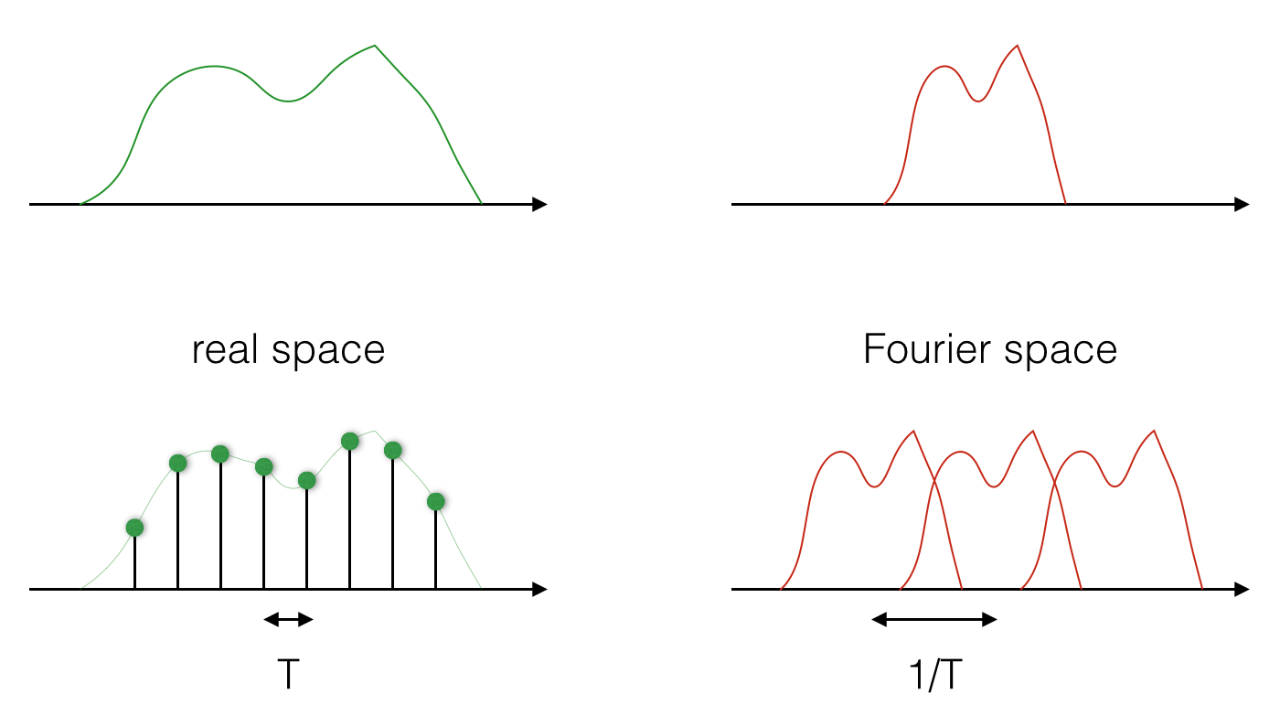
The most important fact about sampling is this: taking samples in real space is the same as repeating the Fourier transform periodically, and the period of repetition is the inverse of the sampling period. Read this again to make sure you understand it. Perhaps the picture below can help:
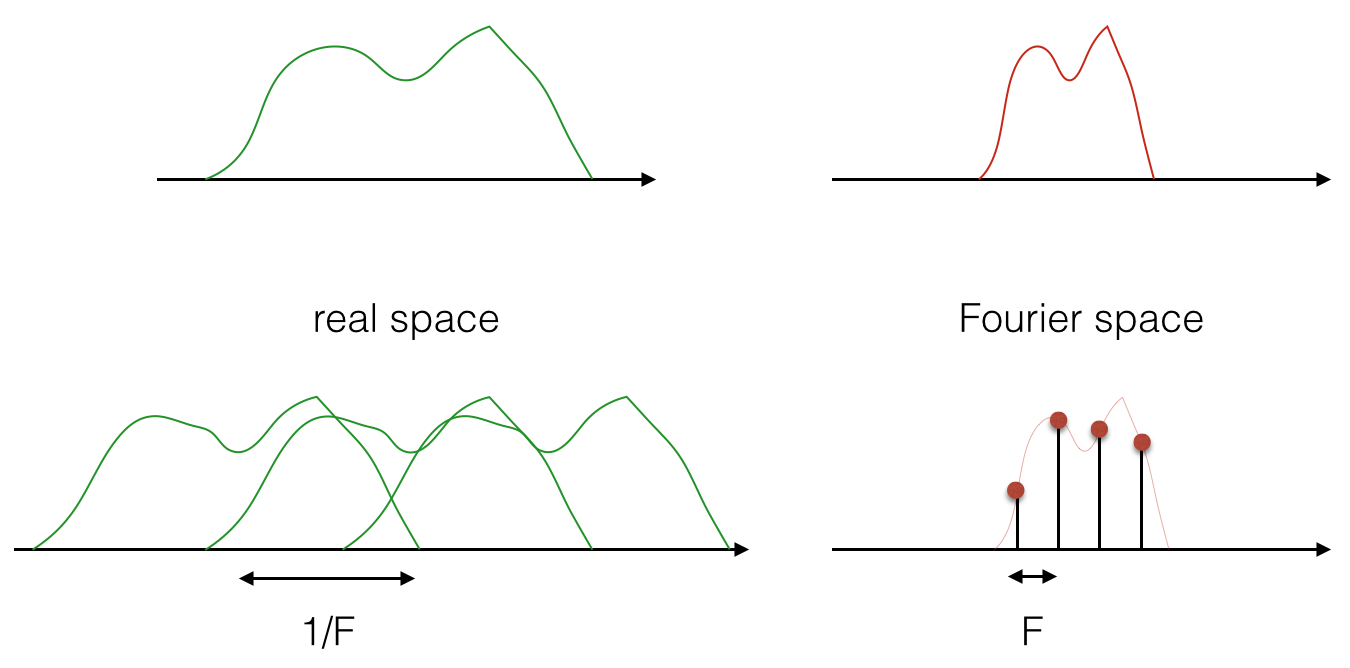
And the image below shows that it is also true the other way round:
Now, the above is true in general for the Fourier transform. But in signal processing and the world of discrete data, we are doing a discrete Fourier transform with the FFT. So in practice, both the real and the Fourier domains are given by samples. This means that they are both sampled, and they are both repeated! See the figure below:
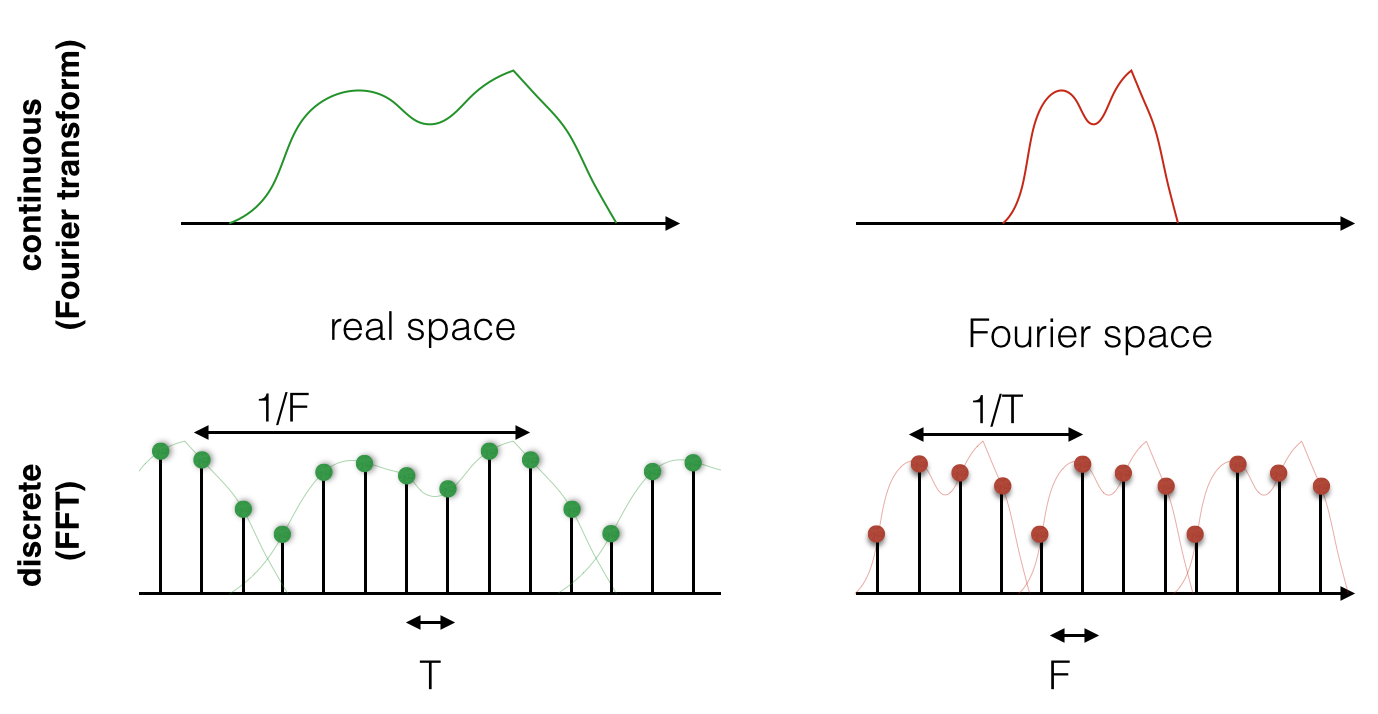
Now, when you run an FFT in Numpy, the repeating pattern is not apparent. That is because the FFT algorithm implicitly considers the signal and its FFT to be periodic (i.e. repeating) and only gives you one period.
How does the above information help us understand sampling? Well, let's simulate a simple signal that consists of the superposition of two cosine functions. We will simulate this signal at high sampling rate (as if it was continuous), and see what happens when we downsample it. Begin by generating the signal:
freq1 = 5.0      # freq in Hz
freq2 = 1.0      # freq in Hz
samp  = 1000.0   # sampling rate in Hz

t = np.arange(0,1,1/samp)  # time (1s of data)
N = len(t)                 # store the number of time points

x = np.cos(2*np.pi*freq1*t) + .5*np.cos(2*np.pi*freq2*t)    # the signal equation
plt.plot(t,x,'.-')
plt.show()
Now remember: this signal is assumed by the FFT to be periodic, so even though it has finite duration, it will be treated by the FFT as if it were repeating, and therefore as if it were a true cosine function.
Let's see what happens when we take subsamples from this signal (make sure you understand all the code below):
F = 50.0         # sub-sampling frequency (Hz)
T = 1/F          # sub-sampling period (sec)
n = int(N*T)     # sub-sampling period (in samples)

z = x[::n]         # sub-sampled signal
y = np.fft.fft(z)  # fft of sub-sampled signal

subN = len(z)  # length of sub-sampled signal


f = np.linspace(0,subN-1,subN)  # vector of frequencies for plotting

plt.plot(f[:subN//2], np.abs(y[:subN//2])) # plot powerspectrum as before
plt.show()
Now change the frequency of sub-sampling and see what happens to
the fourier transform. You should be able to see that as soon as you
drop below 10Hz, you loose the peak at 5Hz in the powerspectrum. Try
to use the ifft function to reconstruct the signal from
its fft and compare it to the almost continuous version.
Example
Now let us look at another concept that we haven't looked at so far: zero padding. We will use the 2D FFT and the cat example to get an understanding of zero padding. First load the image and downsample it by removing every other pixel:
im = mpimg.imread('cat.jpg')
x  = im[::2,::2,0]
plt.imshow(x)
plt.show()
Now let's look at the FFT of this image:
y    = np.fft.fft2(x)
clim = np.quantile(np.abs(y.reshape(-1)),[.01, .99])
plt.imshow(np.fft.fftshift(np.abs(y)), vmin=clim[0], vmax=clim[1])
plt.gray()
plt.show()
Now let us recall the sampling pictures that we showed above. They tell us that repeating the Fourier transform is the same as taking samples in real space. Furthermore, the repeating period is inversely related to the sampling period.
Zero padding means adding zeros on either side of the FFT before reconstructing the signal. Since the Numpy FFT assumes the signal to be periodic, zeropadding is like repeating the signal with increased repeat period, which in the real domain means higher sampling rate. Therefore, zero padding allows us to reconstruct an image at higher resolution than the frequency domain allows us to, and is closely related to the concept of interpolation.
Let's see what the zero padded inverse FFT of the cat looks like:
y = np.fft.fftshift(y)         # we need this before zero padding
z = np.fft.ifft2(y, s=im.shape[:2]) # zero padded ifft
clim = np.quantile(np.abs(z.reshape(-1)), [.01, .99])
plt.imshow(np.abs(z), vmin=clim[0], vmax=clim[1])
plt.show()
Compare to the original image, you should notice strange patterns of "oscillations" caused by the interpolation.
Filtering
Here we will implement a simple linear filter using convolution and the Fourier transform.
Recall that convolution in real space is the same as multiplication in Fourier space, and vice versa. But convolution is more difficult to implement than multiplication, so often it is a good idea to do a Fourier transform of the signal and of the filter, then multiply the two FFTs together, and then do an inverse FFT.
Let's first design a filter. We are going to do this in 2D, so load the cat image if you haven't done that yet.
Now let's create a "moving average" filter (also called the mean filter). This means a box that we are going to run through the image and take local averages.
siz = [3, 3]   # 3x3 box. You can play with changing this
box = np.ones(siz)/9
Now we could create a loop through all the image and for each pixel of the image replace the value by the weighted average within the small box. Instead, we are going to do this via a Fourier transform. First, let's calculate the Fourier transform of the image and the filter:
x = im[:,:,0]
y = np.fft.fft2(x)

f = np.fft.fft2(box, s=x.shape)  # use zeropadding

z = np.fft.ifft2(y*f)  # inverse FFT of the product

clim = np.quantile(np.abs(z.reshape(-1)), [.01, .99])
plt.imshow(np.abs(z), vmin=clim[0], vmax=clim[1])
plt.show()
Beautifully simple no? Imagine doing this with a loop, and having to worry about the edges of the image etc. The effect of a moving average filter is to blur the image, which can be useful for denoising. Try with different filter sizes, what do you notice?
A better behaved filter is the Gaussian filter. It is similar to the mean filter, except that instead of the values in the box being constant, they follow a Gaussian function centered in the middle of the box and with given standard deviation.
Now that you have seen the mean filter, try to implement the Gaussian filter before you click on the answer
Try to use the Gaussian filter to denoise the cat image (add some
noise with the np.random.randn function and then convolve the result with the
Gaussian filter).
Let's now design another type of filter: an edge detection filter. The simplest such filter is to do a derivative, which in discrete terms is simply the difference between adjacent pixels.
Here are simple finite difference filters:
box = [[-1, 1]]          # along x-dimension
box = [[-1],[ 1]]        # along y-dimension
box = [[-1, 0, 1]]       # a slightly better filter along x
box = [[-1],[ 0],[ 1]]   # a slightly better filter along y
Now let's apply these filters to the cat image:
x = im[:,:,0]
y = np.fft.fft2(x)

box = [[-1, 0, 1]] # try with different ones if you have time
f = np.fft.fft2(box, s=x.shape)  # use zeropadding

z = np.fft.ifft2(y*f)  # inverse FFT of the product

clim = np.quantile(np.abs(z.reshape(-1)), [.01, .99])
plt.imshow(np.abs(z), vmin=clim[0], vmax=clim[1])
plt.show()
You should be able to see edges along the x-dimension in the image (similarly along the y dimension if you used the y-derivative filter). These types of operations are extremely widely used in image processing for extracting basic information from images. Other types of filtering operations are also possible (such as non-linear filters), but these can't be implemented with the Fourier transform.
Image reconstruction
Computed Tomography
Image reconstruction means constructing the image of an object from measurements. Here we are going to see two types of image reconstruction which are at the basis of two very popular imaging techniques: The Radon transform, which is at the heart of computed tomography (CT), and the Fourier transform, which is the basis of Magnetic Resonance Imaging (MRI).
You should be quite familiar with the Fourier transform by now, so for a bit of a change, let's examine the Radon transform.
The Radon transform takes an object, and calculates integrals along lines crossing through the object at different angles. The figure below illustrates this process in 2D:
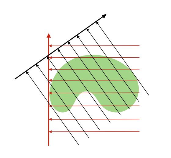
In CT, X-rays are emitted by a source, they then go through an object (typically a body) and get absorbed to various degrees before hitting a detector. The signal that is measured is an integral along a line from the source to the detector that calculates how much absorption there was. So it is easy to see how this relates to the radon transform.
Now, we are faced with the problem of reconstructing the object (body organs), given CT measurements along various angles. The Radon theorem tells us that we can recontruct the object perfectly if we have an infinite number of measurement angles, but in practice this is never the case. So let's see how few measurements we can get away with.
First, we need an object. We are going to remain in 2 dimensions, and we are going to use the most famous image in medical imaging: the Shepp-Logan phantom. This image is so popular that it is included in the skimage's data module, so let's create it:
import skimage.data
im = skimage.data.shepp_logan_phantom()
plt.imshow(im)
plt.gray()
plt.show()
Let's calculate the Radon transform along a single orientation:
import skimage.transform

R = skimage.transform.radon(im, [0])
plt.plot(R)
plt.show()
The above simply sums the values inside the phantom along lines that
are parallel to the x-axis. You can see that by comparing R to
np.sum(im,axis=0).
Now let's look at the Radon transform along more angles and plot the results:
R = skimage.transform.radon(im, np.linspace(0,180,40))   # 40 angles from 0 to 180 degrees
plt.imshow(R)
plt.show()
This funky looking image is your measurement. Now let's calculate an inverse Radon transform and see what the object looks like:
x = skimage.transform.iradon(R, np.linspace(0,180,40))
plt.imshow(x)
plt.show()
The inverse Radon transfrom is also called back-projection. You can clearly see that this back-projection leaves "trails" behind when it tries to reconstruct the object. Try the above with different numbers of projections to get a feel for how many is enough. Note also that the small details in the object require more angles in order to be properly recovered.
In CT, the measurement is actually not exactly the integral of the object along the X-ray beam, but the integral of the "absorption" along the beams. But we will ignore that and pretend that we are measuring the integral of the object's mass. Next we are going to introduce a "metal" artefact. This happens when a patient has an implant inside their body. We can model that by introducing a spike in the original phantom image:
im[200,100] = 100
Now run the radon transform (to simulate the measurement process) and then the inverse radon transform (reconstruction of the object from the measurements). You should be able to see some striking artefacts caused by the simulated metal implant.
R = skimage.transform.radon(im, np.linspace(0,180,100))
x = skimage.transform.iradon(R, np.linspace(0,180,100))
plt.imshow(x, vmin=0, vmax=1)
plt.show()
The Radon transform is related to the Fourier transform via the projection-slice theorem. This theorem states that if you have an object (e.g. in 2D), then projecting the object onto a line is the same as taking a slice through the 2D Fourier transform of the object:
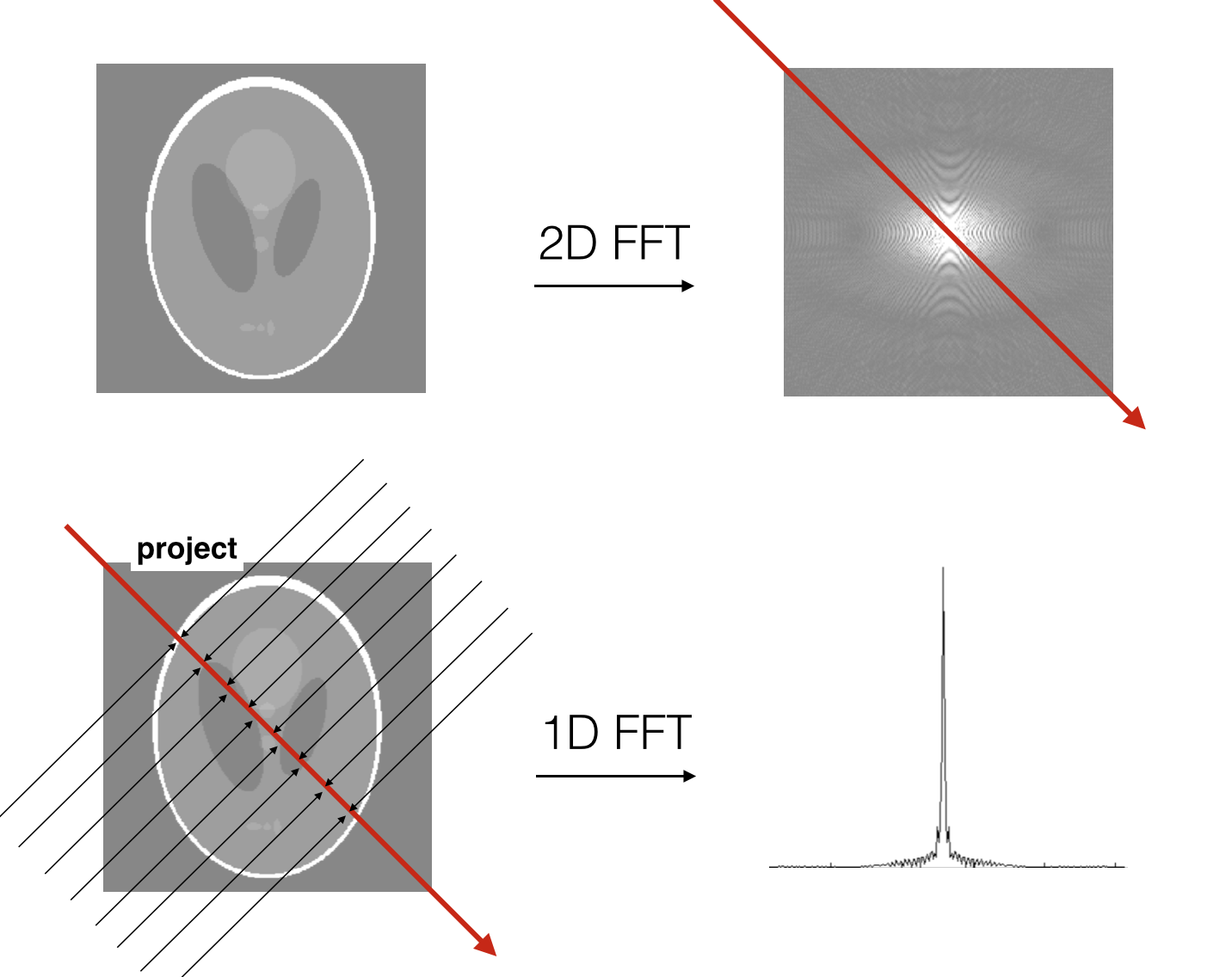
Let us try to verify the projection-slice theorem on the phantom
image. To simplify things, let's just try a projection along either
X or Y axis (which can be done with the sum function in
Numpy).
Answer
The projection-slice theorem therefore tells us that we can measure the entire 2D FFT of an object by calculating the 1D FFT of its projections along different angles. Therefore, we can, with an inverse 2D FFT, reconstruct the object from its Radon transform (i.e. provides a method for performing an inverse Radon transform). As an exercise, you may try to implement the inverse radon transform of an image using the projection-slice theorem and the ifft.
MRI
In MRI, the measurement of an object does not consist in integrals along lines. Instead, we directly measure the Fourier transform of the object. Typically, we measure the 2D Fourier transform of a slice through the object (e.g. in a technique called Echo Planar Imaging).
The Fourier space in MRI is called k-space. You can imagine k-space to be an image, where each pixel is a k-space sample, consisting of a complex number (magnitude and phase). Image reconstruction is then simply implemented with an inverse FFT (but with many twists depending on how sophisticated the measurement is).
Because of time limitations in typical experiments, we can only measure a smallish number of k-space pixels. This has consequences in terms of the quality of the reconstructed image, and many artefacts in MRI come from what happens when we measure k-space.
There are a number of MRI artefacts. In the remainder of this practical, we are going to simulate 3 types of artefacts that are frequent in MRI: Gibb's ringing, ghosting, and T2* blurring.
But first, download this brain and load it into Python:
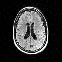
im = skimage.io.imread('brain.bmp')
Remember that in MRI, we measure the FFT of the object, aka
k-space. Let's generate a measured k-space data (and also centre k-space using fftshift):
data = np.fft.fftshift(np.fft.fft2(im))
Gibb's ringing
Gibb's ringing occurs when the frequencies that are sampled in k-space are not sufficiently high (remember: high frequencies are at the edges of k-space, low frequencies at the centre). We simulate this by "cutting" k-space along one of the two axes, as if we didn't have enough time to acquire these data. To exagerate the ringing, we will cut quite a lot of the high frequencies:
K = data[:,112:112+32] # this turns k-space from 256x256 to 256x32
And now reconstruct the object as a full 256x256 (with zero padding, remember?):
x = np.fft.ifft2(K,s=[256,256])
plt.imshow(np.abs(x))    # we typically look at the magnitude
plt.show()
You should be able to see the ringing artefacts along the horizontal axis but not the vertical axis.
Ghosting
Ghosting happens when even and odd k-space lines are intensity modulated differently. We are going to simulate this by taking every other line in k-space and scaling them by 80 percent:
K = data.copy()
K[::2,:] = 0.8*K[::2,:]
x = np.fft.ifft2(K)
plt.imshow(np.abs(x))
plt.show()
You can see that the image gets "duplicated" and overlaps with itself along the dimension where we did the intensity modulation. Try along the other dimension now:
K = data.copy()
K[:,::2] = 0.8*K[:,::2]
x = np.fft.ifft2(K)
plt.imshow(np.abs(x))
plt.show()
Why does this happen? One way to understand this is to notice that modulating every other slice of the k-space data is like taking the original k-space data (unmodulated), and adding to it k-space data that is sampled at 2 pixel intervals (or rather adding -0.2 times that). Now remember that sampling in one space is the same as repeating in the other space. Sampling with a period of 2 pixels is the same as repeating with a period of N/2 pixels in the other space. So therefore, the reconstructed image is like the original images, plus a "ghost" image that is repeated with cycles of N/2 pixels.
T2* blurring
The final MRI artefact that we will look at is T2* blurring. This particular artefact is due to the fact that when we acquire k-space data, the signal that we base our measurement on decays over time, with a time constant called T2* (don't ask why!).
Typically, we acquire k-space, say, from the bottom to the top, so we will simulate an intensity drop along that direction:
T2star = 20            # milliseconds
Ttotal = 100           # time it takes to "read" k-space
N      = data.shape[0] # number of pixels

K = data.copy()
for i in range(K.shape[1]):
    K[:,i] = K[:,i]*np.exp(-np.linspace(0,Ttotal,N)/T2star)
Now let's reconstruct the object and see what happened:
x = np.fft.ifft2(K)
plt.imshow(np.abs(x))
plt.show()
You should be able to see some blurring along the vertical axis. The shorter the value of T2* is, the more blurring there is (try this!).
Why does this happen? The easiest way to understand this is to consider that multiplying the k-space trajectory by an exponential decay is the same as doing a convolution of the image space with the Fourier transform of the exponential (which is called a Lorentzian function). This convolution operation effectively blurs the image.
Ok, well done for getting to the end of the practical. If you have gone through it very fast and have plenty of time left, maybe you can explore other possible sources of k-space MRI artefacts and try to predict what happens to the object before you check with the inverse FFT. It should be fun!
The End.
Created by Saad Jbabdi (saad@fmrib.ox.ac.uk)